library(tidyverse)
library(caret)
library(glmnet)Exercise 5C - Solutions: Elastic Net Regression
Elastic Net Regression
- Load the R packages needed for analysis:
- Load in the dataset
Obt_Perio_ML.Rdataand inspect it.
load(file = "../data/Obt_Perio_ML.Rdata")- Do some basic summary statistics and distributional plots to get a feel for the data. Which types of variables do we have?
# Reshape data to long format for ggplot2
long_data <- optML %>%
  dplyr::select(where(is.numeric)) %>%
  pivot_longer(cols = everything(),
               names_to = "variable",
               values_to = "value")

# Plot histograms for each numeric variable in one grid
ggplot(long_data, aes(x = value)) +
  geom_histogram(binwidth = 0.5, fill = "#9395D3", color ='grey30') +
  facet_wrap(~ variable, scales = "free") +
  theme_minimal()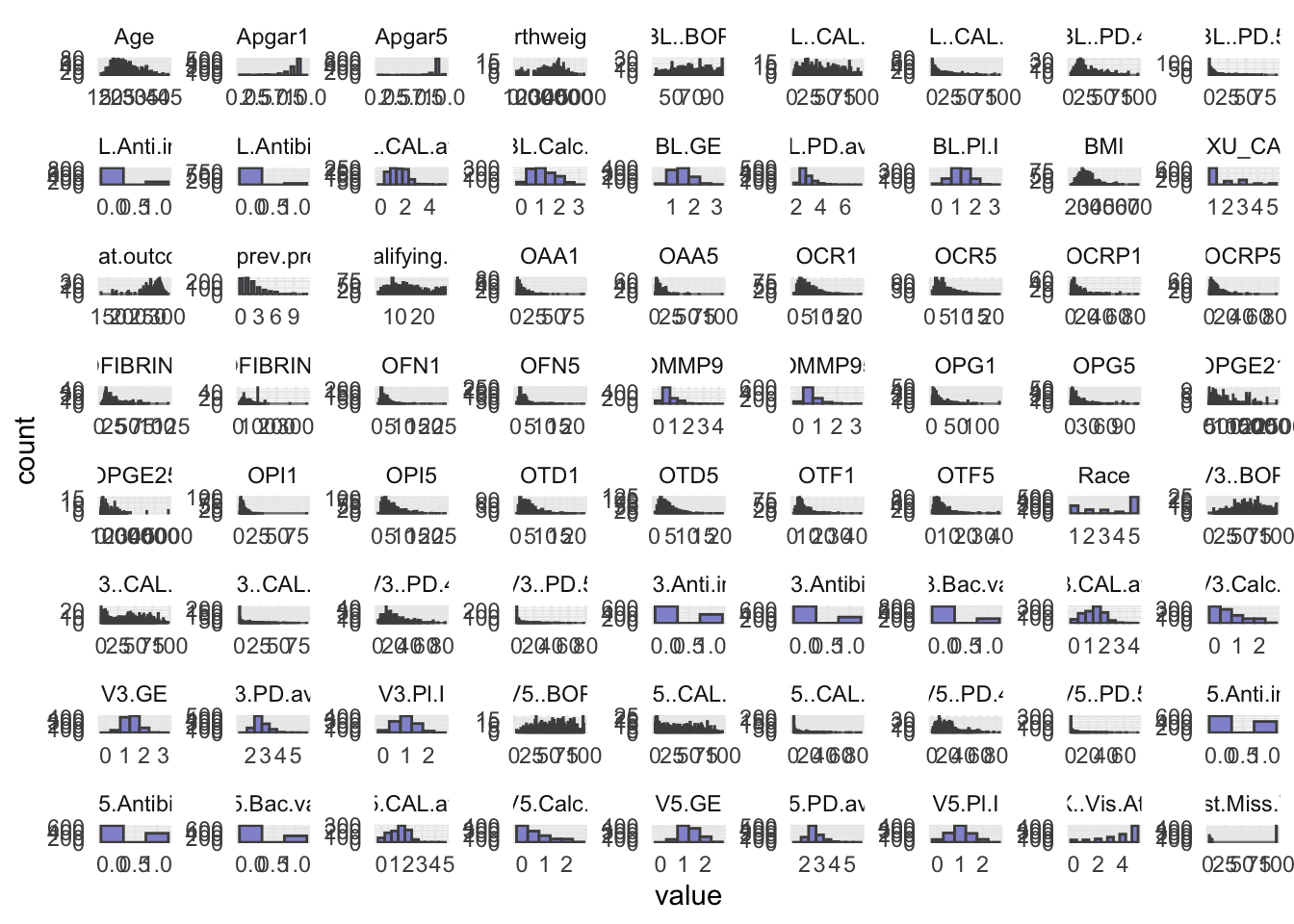
- Some of the numeric variables are actually categorical. We have identified them in the
facColsvector below. Change their type from numeric to character.
facCols <- c("Race",
             "ETXU_CAT5",
             "BL.Anti.inf",
             "BL.Antibio",
             "V3.Anti.inf",
             "V3.Antibio",
             "V3.Bac.vag",
             "V5.Anti.inf",
             "V5.Antibio",
             "V5.Bac.vag",
             "X..Vis.Att")


optML <- optML %>%
  mutate(across(all_of(facCols), as.character))

head(optML)
# A tibble: 6 × 89
PID Apgar1 Apgar5 Birthweight GA.at.outcome Any.SAE. Clinic Group Age
<chr> <dbl> <dbl> <dbl> <dbl> <chr> <chr> <chr> <dbl>
1 P10 9 9 3107 278 No NY C 30
2 P170 9 9 3040 286 No MN C 20
3 P280 8 9 3370 282 No MN T 29
4 P348 9 9 3180 275 No KY C 18
5 P402 8 9 2615 267 No KY C 18
6 P209 8 9 3330 284 No MN C 18
# ℹ 80 more variables: Race <chr>, Education <chr>, Public.Asstce <chr>,
# BMI <dbl>, Use.Tob <chr>, N.prev.preg <dbl>, Live.PTB <chr>,
# Any.stillbirth <chr>, Any.live.ptb.sb.sp.ab.in.ab <chr>,
# EDC.necessary. <chr>, N.qualifying.teeth <dbl>, BL.GE <dbl>, BL..BOP <dbl>,
# BL.PD.avg <dbl>, BL..PD.4 <dbl>, BL..PD.5 <dbl>, BL.CAL.avg <dbl>,
# BL..CAL.2 <dbl>, BL..CAL.3 <dbl>, BL.Calc.I <dbl>, BL.Pl.I <dbl>,
# V3.GE <dbl>, V3..BOP <dbl>, V3.PD.avg <dbl>, V3..PD.4 <dbl>, …- As you will use the response
Preg.ended...37.wk, you should remove the other five possible outcome variables measures from your dataset. You will need to take out one more variable from the dataset before modelling, figure out which one and remove it.
optML <- optML %>%
dplyr::select(-c(Apgar1, Apgar5, GA.at.outcome, Birthweight, Any.SAE., PID))- Elastic net regression can be sensitive to large differences in the range of numeric/integer variables, as such these variables should be scaled. Scale all numeric/integer variables in your dataset.
optML <- optML %>%
mutate(across(where(is.numeric), scale))- Split your dataset into train and test set, you should have 70% of the data in the training set and 30% in the test set. How you chose to split is up to you, BUT afterwards you should ensure that for the categorical/factor variables all levels are represented in both sets.
# Set seed
set.seed(123)

idx <- createDataPartition(optML$Preg.ended...37.wk, p = 0.7, list = FALSE)
train <- optML[idx, ]
test  <- optML[-idx, ]
# Train Split
train[,-1] %>%
dplyr::select(where(is.character)) %>%
pivot_longer(everything(), names_to = "Variable", values_to = "Level") %>%
dplyr::count(Variable, Level, name = "Count")# A tibble: 60 × 3
Variable Level Count
<chr> <chr> <int>
1 Any.live.ptb.sb.sp.ab.in.ab No 304
2 Any.live.ptb.sb.sp.ab.in.ab Yes 397
3 Any.stillbirth No 620
4 Any.stillbirth Yes 81
5 BL.Anti.inf 0 601
6 BL.Anti.inf 1 100
7 BL.Antibio 0 643
8 BL.Antibio 1 58
9 Bact.vag No 606
10 Bact.vag Yes 95
# ℹ 50 more rows## Test Split
# test[,-1] %>%
# dplyr::select(where(is.character)) %>%
# pivot_longer(everything(), names_to = "Variable", values_to = "Level") %>%
# dplyr::count(Variable, Level, name = "Count")- After dividing into train and test set pull out the outcome variable,
Preg.ended...37.wk, into its own vector for both datasets. Name thesey_trainandy_test.
y_train <- train %>%
  pull(Preg.ended...37.wk)


y_test <- test %>%
pull(Preg.ended...37.wk)- Remove the outcome variable,
Preg.ended...37.wk, from the train and test set, as we should obviously not use this for training.
train <- train %>%
  dplyr::select(-Preg.ended...37.wk)


test <- test %>%
  dplyr::select(-Preg.ended...37.wk)
You will employ the package glmnet to perform Elastic Net Regression. The main function from this package is glmnet() which we will use to fit the model. Additionally, you will also perform cross validation with cv.glmnet() to obtain the best value of the model hyper-parameter, lambda (\(λ\)).
As we are working with a mix of categorical and numerical predictors, it is advisable to dummy-code the variables. You can easily do this by creating a model matrix for both the test and train set.
- Create the model matrix needed for input to
glmnet()andcv.glmnet().
modTrain <- model.matrix(~ ., data = train)
modTest <- model.matrix(~ ., data = test)- Create your Elastic Net Regression model with
glmnet().
EN_model <- glmnet(modTrain, y_train, alpha = 0.5, family = "binomial")- Use
cv.glmnet()to attain the best value of the hyperparameter lambda (\(λ\)). Remember to set a seed for reproducible results.
set.seed(123)
cv_model <- cv.glmnet(modTrain, y_train, alpha = 0.5, family = "binomial")- Plot all the values of lambda tested during cross validation by calling
plot()on the output of yourcv.glmnet(). Extract the best lambda value from thecv.glmnet()model and save it as an object.
plot(cv_model)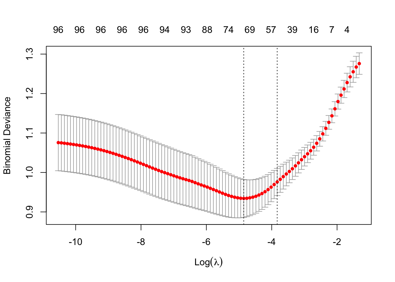
bestLambda <- cv_model$lambda.minNow, let’s see how well your model performed.
- Predict if an individual is likely to give birth before the 37th week using your model and your test set. See pseudo-code below
y_pred <- predict(EN_model, s = bestLambda, newx = modTest, type = 'class')- Just like for the logistic regression model you can calculate the accuracy of the prediction by comparing it to
y_testwithconfusionMatrix(). Do you have a good accuracy? N.B look at the 2x2 contingency table, what does it tell you?
y_pred <- as.factor(y_pred)

caret::confusionMatrix(y_pred, y_test)
Confusion Matrix and Statistics
Reference
Prediction 0 1
0 186 39
1 14 60
Accuracy : 0.8227
95% CI : (0.7746, 0.8643)
No Information Rate : 0.6689
P-Value [Acc > NIR] : 1.937e-09
Kappa : 0.5726
Mcnemar's Test P-Value : 0.0009784
Sensitivity : 0.9300
Specificity : 0.6061
Pos Pred Value : 0.8267
Neg Pred Value : 0.8108
Prevalence : 0.6689
Detection Rate : 0.6221
Detection Prevalence : 0.7525
Balanced Accuracy : 0.7680
'Positive' Class : 0
- Lastly, let’s extract the variables which were retained in the model (e.g. not penalized out). We do this by calling the coefficient with
coef()on our model. See pseudo-code below.
coeffs <- coef(EN_model, s = bestLambda)

# Convert coefficients to a data frame for easier viewing
coeffsDat <- as.data.frame(as.matrix(coeffs)) %>%
rownames_to_column(var = 'VarName')- Make a plot that shows the absolute importance of the variables retained in your model. This could be a barplot with variable names on the y-axis and the length of the bars denoting absolute size of coefficient.
# Make dataframe ready for plotting, remove intercept and coeffcients that are zero
coeffsDat <- coeffsDat %>%
  mutate(AbsImp = abs(s0)) %>%
  arrange(AbsImp) %>%
  mutate(VarName = factor(VarName, levels=VarName)) %>%
  filter(AbsImp > 0 & VarName != "(Intercept)")


# Plot last 20 variables with the greatest importance
ggplot(coeffsDat[71:51, ], aes(x = VarName, y = AbsImp)) +
  geom_bar(stat = "identity", fill = "#9395D3") +
  coord_flip() +
  labs(title = "Feature Importance for Elastic Net",
       x = "Features",
       y = "Absolute Coefficients") +
  theme_classic()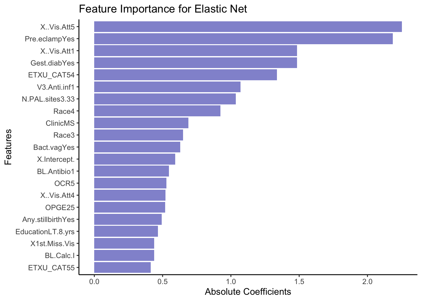
- Now repeat what you just did above, but this time instead of using
Preg.ended...37.wkas outcome, try using a continuous variable, such asGA.at.outcome. N.B remember this means that you should evaluate the model using the RMSE and a scatter plot instead of the accuracy!