library(tidyverse)
library(readxl)Solution 1: Data Cleaning
Getting started
- Load packages.
- Load in the
diabetes_clinical_toy_messy.xlsxdata set.
diabetes_clinical <- read_excel('../data/diabetes_clinical_toy_messy.xlsx')
head(diabetes_clinical)
# A tibble: 6 × 9
ID Sex Age BloodPressure BMI PhysicalActivity Smoker Diabetes
<dbl> <chr> <dbl> <dbl> <dbl> <dbl> <chr> <dbl>
1 9046 Male 34 84 24.7 93 Unknown 0
2 51676 Male 25 74 22.5 102 Unknown 0
3 31112 Male 30 0 32.3 75 Former 1
4 60182 Male 50 80 34.5 98 Unknown 1
5 1665 Female 27 60 26.3 82 Never 0
6 56669 Male 35 84 35 58 Smoker 1
# ℹ 1 more variable: Serum_ca2 <dbl>Explore the data
- How many missing values (NA’s) are there in each column.
colSums(is.na(diabetes_clinical)) ID Sex Age BloodPressure
0 0 3 0
BMI PhysicalActivity Smoker Diabetes
3 0 0 0
Serum_ca2
0 - Check the ranges and distribution of each of the numeric variables in the dataset. Do any values seem weird or unexpected? Extract summary statistics on these, e.g. means and standard deviation.
For the numerical variables we’ll plot and check the range:
# Range
range(diabetes_clinical$Age, na.rm = TRUE)
[1] 21 81# Histogram
diabetes_clinical$Age %>% hist()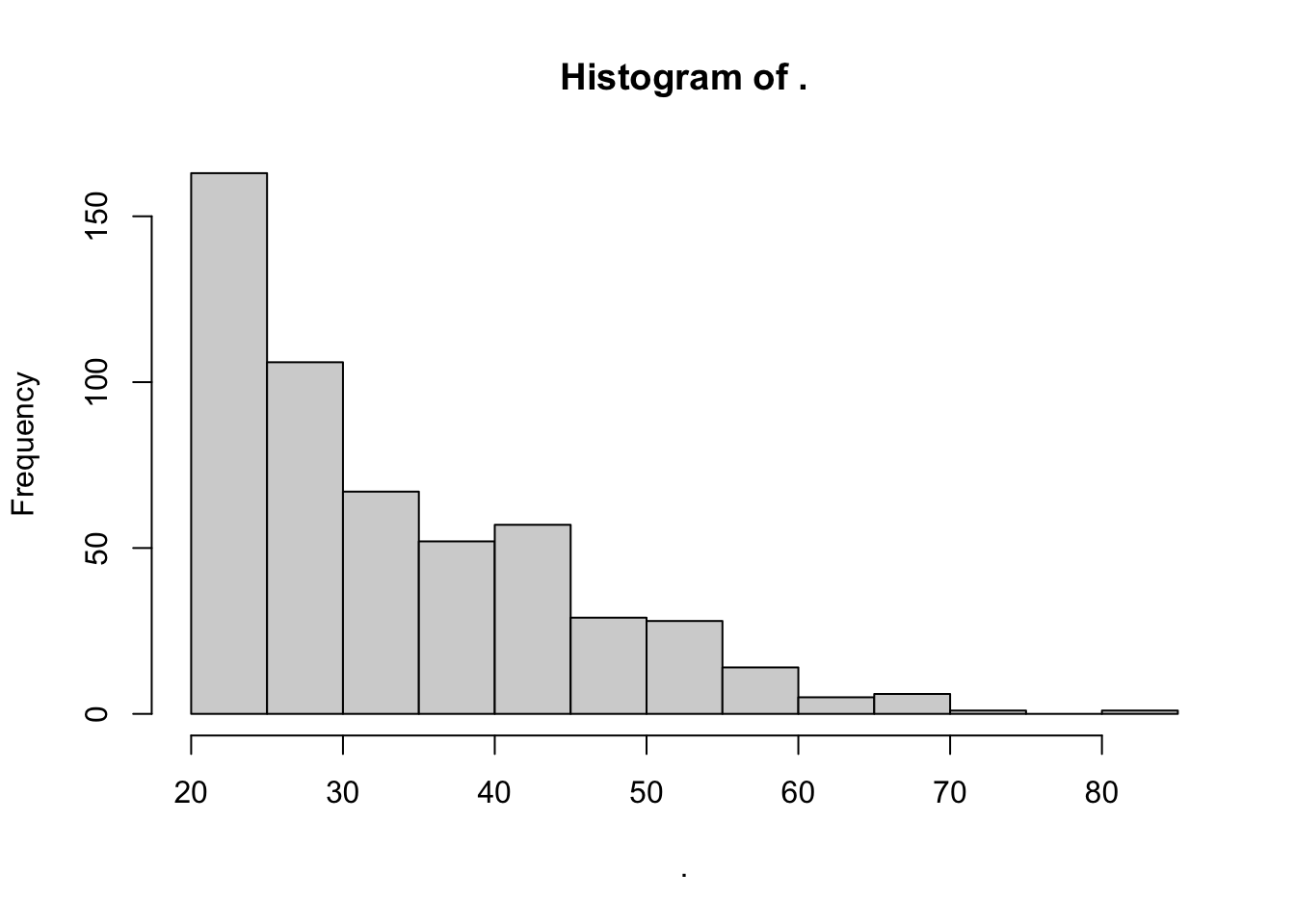
# ggplot2 boxplot
diabetes_clinical %>%
  ggplot(aes(y = Age, x = 1)) +
  geom_boxplot(fill="steelblue") +
  theme_minimal()
Warning: Removed 3 rows containing non-finite outside the scale range
(`stat_boxplot()`).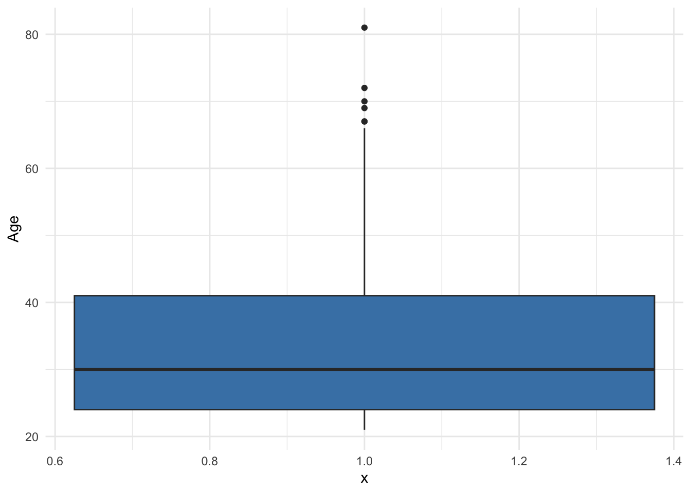
Odd: Some BloodPressure values are 0.
range(diabetes_clinical$BloodPressure, na.rm = TRUE)[1] 0 114diabetes_clinical %>%
ggplot(aes(x = BloodPressure)) +
geom_histogram(color='black', fill='grey') +
theme_minimal()`stat_bin()` using `bins = 30`. Pick better value with `binwidth`.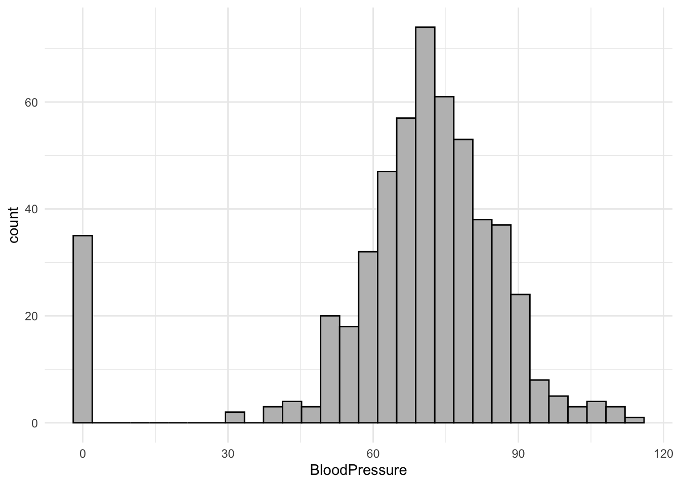
Odd: Some BMI values are 0.
range(diabetes_clinical$BMI, na.rm = TRUE)[1] 0.0 57.1diabetes_clinical %>%
ggplot(aes(y = BMI, x = 1)) +
geom_violin(fill="#ADC698") +
geom_point() +
theme_minimal()Warning: Removed 3 rows containing non-finite outside the scale range
(`stat_ydensity()`).Warning: Removed 3 rows containing missing values or values outside the scale range
(`geom_point()`).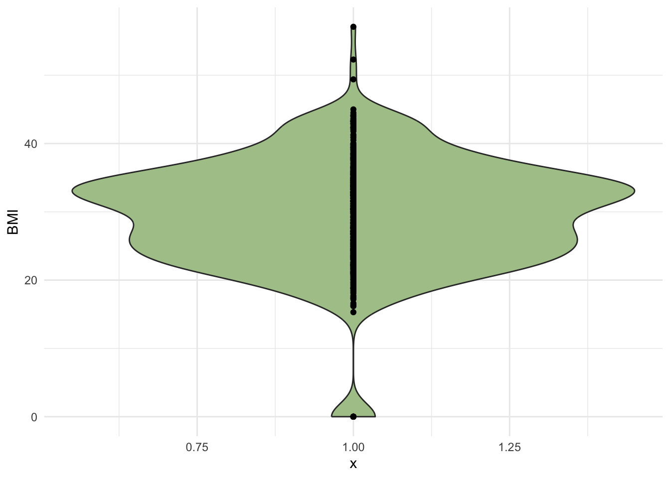
range(diabetes_clinical$PhysicalActivity, na.rm = TRUE)[1] 19 177diabetes_clinical %>%
ggplot(aes(y = PhysicalActivity)) +
geom_boxplot(color='black', fill='grey') +
theme_minimal()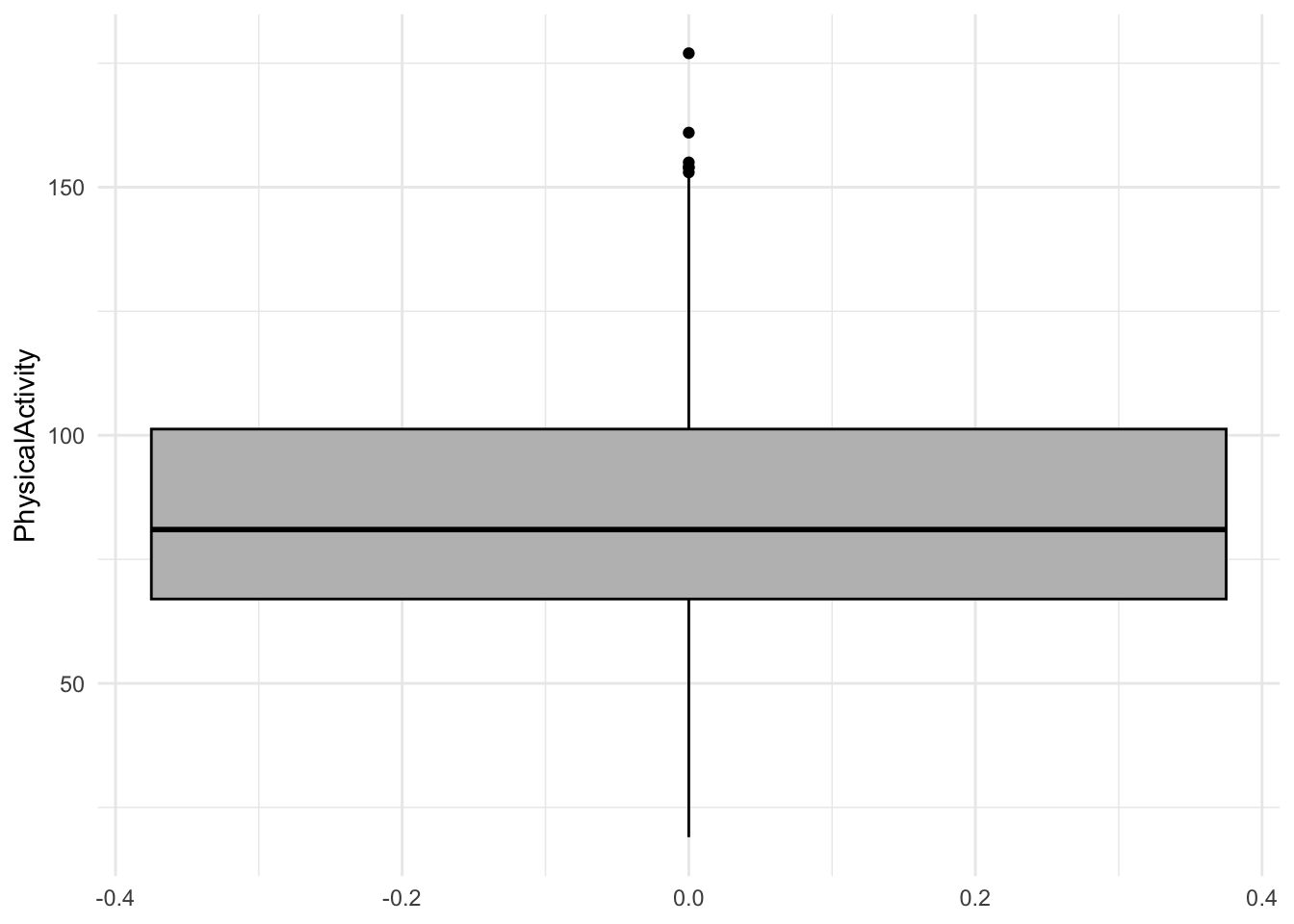
range(diabetes_clinical$Serum_ca2, na.rm = TRUE)[1] 8.7 10.2diabetes_clinical %>%
ggplot(aes(x = Serum_ca2)) +
geom_histogram(color='black', fill='#ADC698') +
theme_minimal()`stat_bin()` using `bins = 30`. Pick better value with `binwidth`.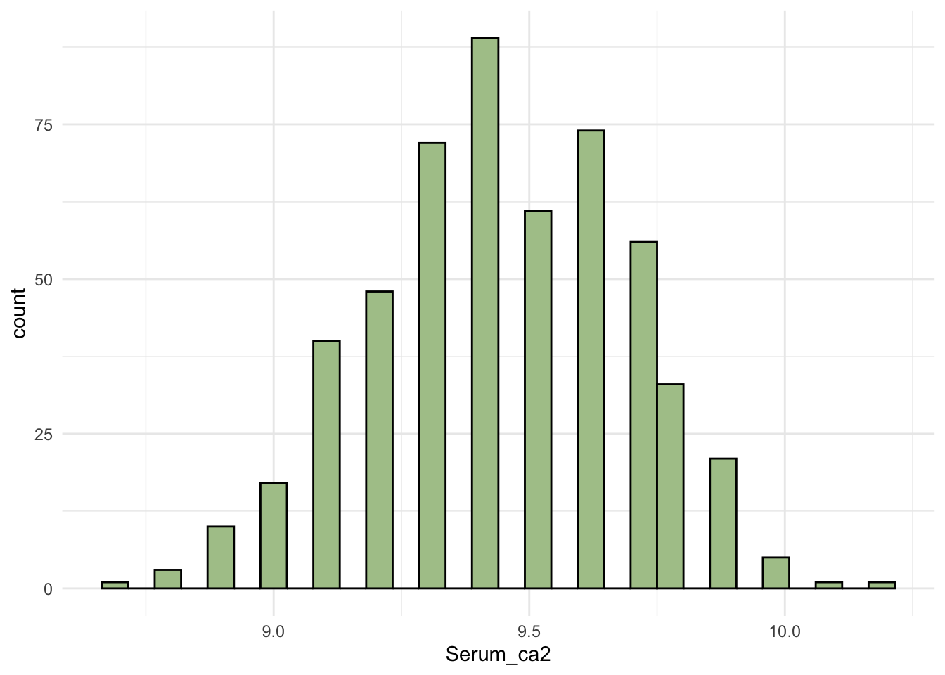
- Some variables in the dataset are categorical or factor variables. Figure out what levels these have and how many observations there are for each level.
For the categorical variables we can use table() (or if you prefer, count()):
The Sex values are not consistent.
table(diabetes_clinical$Sex)
Female FEMALE   male   Male
291 2 2 237 table(diabetes_clinical$Smoker)
 Former   Never  Smoker Unknown
132 159 162 79 table(diabetes_clinical$Diabetes)
  0   1
267 265
Clean up the data
Now that we have had a look at the data, it is time to correct fixable mistakes and remove observations that cannot be corrected.
Consider the following:
What should we do with the rows that contain NA’s? Do we remove them or keep them?
Which odd things in the data can we correct with confidence and which cannot?
Are there zeros in the data? Are they true zeros or errors?
Do you want to change any of the classes of the variables?
- Make a clean version of the dataset according to your considerations.
TipHint
Have a look at BloodPressure, BMI, and Sex.
My considerations:
When modelling, rows with NA’s in the variables we want to model should be removed as we cannot model on NAs. Since there are only NA’s in
AgeandBMI, the rows can be left until we need to do a model with these columns.The different spellings in
Sexshould be regularized so that there is only one spelling for each category. Since most rows have the first letter as capital letter and the remaining letter as lowercase we will use that.There are zeros in
BMIandBloodPressure. These are considered false zeros as is does not make sense that these variables have a value of 0.
Check number of rows before cleaning.
nrow(diabetes_clinical)[1] 532Cleaning data according to considerations.
diabetes_clinical_clean <- diabetes_clinical %>%
  mutate(Sex = str_to_title(Sex)) %>%
  filter(BMI != 0, BloodPressure != 0)
Check the variables that were altered
# Unique sexes now
diabetes_clinical_clean$Sex %>% unique()
[1] "Male" "Female"# Range of BMI and blood pressure
range(diabetes_clinical_clean$BMI, na.rm = TRUE)[1] 15.3 57.1range(diabetes_clinical_clean$BloodPressure, na.rm = TRUE)[1] 30 114Check number of rows after cleaning.
nrow(diabetes_clinical_clean)[1] 490Metadata
- There is some metadata to accompany the dataset you have just cleaned in
diabetes_meta_toy_messy.csv. This is a csv file, not an excel sheet, so you need to use theread_delim()function to load it. Load in the dataset and inspect it.
diabetes_meta <- read_delim('../data/diabetes_meta_toy_messy.csv')
head(diabetes_meta)
# A tibble: 6 × 3
ID Married Work
<dbl> <chr> <chr>
1 48368 Yes Private
2 36706 No Public
3 32729 Yes Private
4 48272 Yes Private
5 9404 Yes Private
6 16934 Yes Self-employed7.1. How many missing values (NA’s) are there in each column.
colSums(is.na(diabetes_meta)) ID Married Work
0 0 0 7.2. Check the distribution of each of the variables. Consider that the variables are of different classes. Do any of the distributions seam odd to you?
For the categorical variables:
table(diabetes_meta$Married)
  No  No   Yes Yes
178 1 332 4 table(diabetes_meta$Work)
      Private        Public       Retired Self-employed
          273           150             6            86
By investigating the unique values of the Married variable we see that some of the values have whitespace.
unique(diabetes_meta$Married)[1] "Yes" "No" "Yes " "No " 7.3. Make a clean version of the dataset according to your considerations.
My considerations:
- The
Marriedvariable has whitespace in the some of the values. The values “Yes” and “Yes” will be interpreted as different values. We can confidently remove all the whitespaces in this variable.
Check number of rows before cleaning.
nrow(diabetes_meta)[1] 515diabetes_meta_clean <- diabetes_meta %>%
mutate(Married = str_trim(Married))Check the unique marital status now.
unique(diabetes_meta_clean$Married)[1] "Yes" "No" Check number of rows after cleaning.
nrow(diabetes_meta_clean)[1] 515Join the datasets
Consider which variable the datasets should be joined on.
Consider how you want to join the datasets. Do you want to use
full_join,inner_join,left_joinandrigth_join?
The joining variable must be the same type in both datasets.
- Join the cleaned versions of the clinical and metadataset by the variable and with the function you considered above.
# We use inner_join to have as few NAs as possiable
diabetes_join <- diabetes_clinical_clean %>%
  inner_join(diabetes_meta_clean, by = 'ID')

nrow(diabetes_join)
[1] 474- How many rows does the joined dataset have? Explain how the join-function you used resulted in the given number of rows.
# Because we used `full_join`, all the unique IDs across both data sets are kept.
c(diabetes_clinical_clean$ID, diabetes_meta_clean$ID) %>%
  unique() %>%
  length()
[1] 531nrow(diabetes_join)[1] 474Manipulate some strings
When we look at the column Work, we can see that we have three levels Public, Private and Self-employed. Some special characters, including: - / \[\] (), etc. can sometimes prove problematic in variable names, as they are also used for operations in R. For example, are dashes (-) used to indicate a contrast in some functions.
- To avoid potential issues in downstream analysis, change the
Workvariable so thatSelf-employedbecomesSelfEmployed.
diabetes_join <- diabetes_join %>%
  mutate(Work = str_replace_all(Work, '-e', 'E'))

table(diabetes_join$Work)
     Private       Public      Retired SelfEmployed
         252          141            4           77
Additionally, we are not so happy with the fact that the ID is simply denoted by a number. The reason for this is that if we write out our dataset and read it in again (which we will do later), R will think it is a numeric or integer variable.
- Add the string
ID_in front of the number and convert it to a factor variable.
diabetes_join <-  diabetes_join %>%
  mutate(ID = paste0("ID_", as.factor(ID)))

head(diabetes_join$ID)
[1] "ID_34120" "ID_27458" "ID_70630" "ID_13861" "ID_68794" "ID_64778"- Export the joined dataset. Think about which directory you want to save the file in.
writexl::write_xlsx(diabetes_join, '../data/exercise1_diabetes_join.xlsx')