library(tidyverse)
library(glmnet)
library(MASS)
library(caret)Presentation 5C: Modelling in R - Elastic Net Regression
Penalized Regression
Elastic Net regression is part of the family of penalized regressions, which also includes Ridge regression and LASSO regression. Penalized regressions are useful when dealing with many predictors (high-dimensional data), as they help eliminate less informative ones while retaining the important predictors.
If you are interested in knowing more about penalized regressions, you can have a look at this excellent tutorial from Datacamp.
In linear regression, we estimate the relationship between predictors \(X\) and an outcome \(y\) using parameters \(β\), chosen to minimize the residual sum of squares (RSS). Two key properties of these \(β\) estimates are bias (the difference between the true parameter and the estimate) and variance (how much the estimates vary across different samples). While OLS gives unbiased estimates, it can suffer from high variance - especially when predictors are numerous or highly correlated — leading to poor predictions.
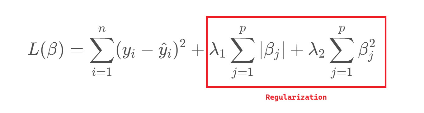
To address this, we can introduce regularization, which slightly biases the estimates in exchange for reduced variance and improved predictive performance. This trade-off is essential: as model complexity grows, variance increases and bias decreases, so regularization helps find a better balance between the two.
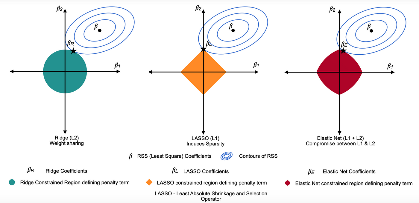
Ridge Regression = L2 penalty (adds the sum of the squares of the coefficients to the loss function). It discourages large coefficients by penalizing their squared magnitudes, shrinking them towards zero. This reduces overfitting while keeping all variables in the model.
Lasso Regression = L1 penalty (adds the sum of the absolute values of the coefficients to the loss function). This penalty encourages sparsity, causing some coefficients to become exactly zero for large \(λ\), thereby performing variable selection.
Elastic Net combines L1 and L2 penalties to balance variable selection and coefficient shrinkage. One of the key advantages of Elastic Net over other types of penalized regression is its ability to handle multicollinearity and situations where the number of predictors exceeds the number of observations.
Lambda, \((λ)\), controls the strength of the penalty. As \(λ\) increases, variance decreases and bias increases, raising the key question: how much bias are we willing to accept to reduce variance?
Elastic Net regression
Load the R packages needed for analysis:
For this exercise we will use a dataset from patients with Heart Disease. Information on the columns in the dataset can be found here.
HD <- read_csv("../data/HeartDisease.csv")

head(HD)
# A tibble: 6 × 14
age sex chestPainType restBP chol fastingBP restElecCardio maxHR
<dbl> <dbl> <dbl> <dbl> <dbl> <dbl> <dbl> <dbl>
1 52 1 0 125 212 0 1 168
2 53 1 0 140 203 1 0 155
3 70 1 0 145 174 0 1 125
4 61 1 0 148 203 0 1 161
5 62 0 0 138 294 1 1 106
6 58 0 0 100 248 0 0 122
# ℹ 6 more variables: exerciseAngina <dbl>, STdepEKG <dbl>,
# slopePeakExST <dbl>, nMajorVessels <dbl>, DefectType <dbl>,
# heartDisease <dbl>Firstly, let’s convert some of the variables that are encoded as numeric datatypes but should be factors:
facCols <- c("sex",
             "chestPainType",
             "fastingBP",
             "restElecCardio",
             "exerciseAngina",
             "slopePeakExST",
             "DefectType",
             "heartDisease")


HD <- HD %>%
  mutate_if(names(.) %in% facCols, as.factor)

head(HD)
# A tibble: 6 × 14
age sex chestPainType restBP chol fastingBP restElecCardio maxHR
<dbl> <fct> <fct> <dbl> <dbl> <fct> <fct> <dbl>
1 52 1 0 125 212 0 1 168
2 53 1 0 140 203 1 0 155
3 70 1 0 145 174 0 1 125
4 61 1 0 148 203 0 1 161
5 62 0 0 138 294 1 1 106
6 58 0 0 100 248 0 0 122
# ℹ 6 more variables: exerciseAngina <fct>, STdepEKG <dbl>,
# slopePeakExST <fct>, nMajorVessels <dbl>, DefectType <fct>,
# heartDisease <fct>Let’s do some summary statistics to have a look at the variables we have in our dataset. Firstly, the numeric columns. We can get a quick overview of variable distributions and ranges with some histograms.
# Reshape data to long format for ggplot2
long_data <- HD %>%
  dplyr::select(where(is.numeric)) %>%
  pivot_longer(cols = everything(),
               names_to = "variable",
               values_to = "value")

head(long_data)
# A tibble: 6 × 2
variable value
<chr> <dbl>
1 age 52
2 restBP 125
3 chol 212
4 maxHR 168
5 STdepEKG 1
6 nMajorVessels 2# Plot histograms for each numeric variable in one grid
ggplot(long_data,
aes(x = value)) +
geom_histogram(binwidth = 0.5, fill = "#9395D3", color ='grey30') +
facet_wrap(vars(variable), scales = "free") +
theme_minimal()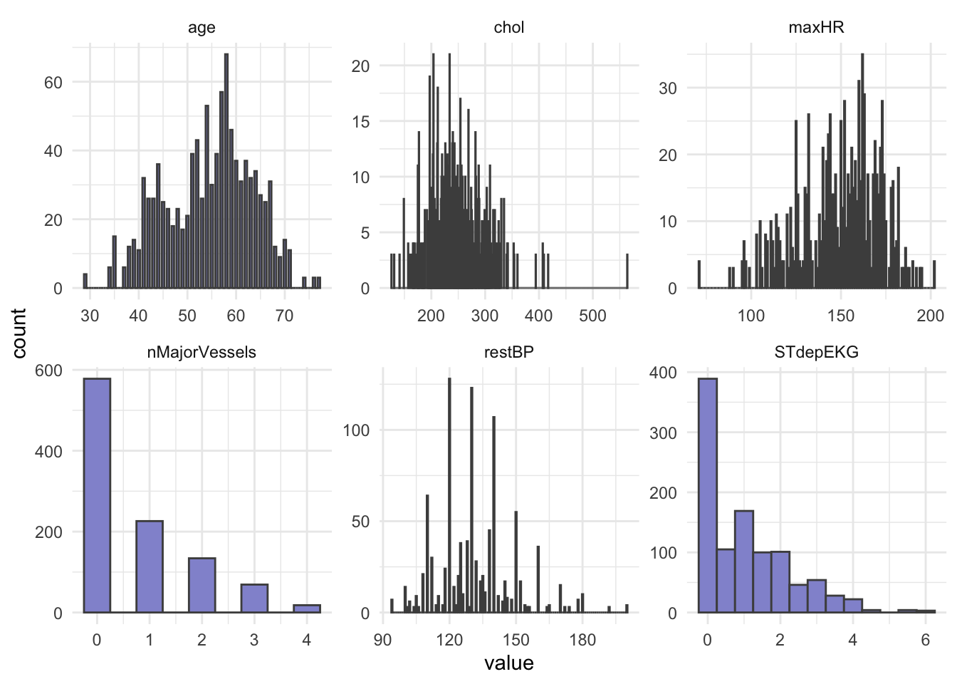
In opposition to hypothesis tests and classic linear regression, penalized regression has no assumption that predictors or model residuals, must be normally distributed. It does however still assume that the relationship between predictors and the outcome is linear and that observations are independent from one another.
Importantly, penalized regression can be sensitive to large differences in the range of numeric/integer variables and it does not like missing values, so lets remove missing (if any) and scale our numeric variables.
Question: What happens to the data when it is scaled?
HD_EN <- HD %>%
  drop_na(.)
HD_EN <-HD %>%
mutate(across(where(is.numeric), scale))
head(HD_EN)# A tibble: 6 × 14
age[,1] sex chestPainType restBP[,1] chol[,1] fastingBP restElecCardio
<dbl> <fct> <fct> <dbl> <dbl> <fct> <fct>
1 -0.268 1 0 -0.377 -0.659 0 1
2 -0.158 1 0 0.479 -0.833 1 0
3 1.72 1 0 0.764 -1.40 0 1
4 0.724 1 0 0.936 -0.833 0 1
5 0.834 0 0 0.365 0.930 1 1
6 0.393 0 0 -1.80 0.0388 0 0
# ℹ 7 more variables: maxHR <dbl[,1]>, exerciseAngina <fct>,
# STdepEKG <dbl[,1]>, slopePeakExST <fct>, nMajorVessels <dbl[,1]>,
# DefectType <fct>, heartDisease <fct>Now, let’s check the balance of the categorical/factor variables.
HD_EN %>%
  dplyr::select(where(is.factor)) %>%
  pivot_longer(everything(), names_to = "Variable", values_to = "Level") %>%
  dplyr::count(Variable, Level, name = "Count")
# A tibble: 22 × 3
Variable Level Count
<chr> <fct> <int>
1 DefectType 0 7
2 DefectType 1 64
3 DefectType 2 544
4 DefectType 3 410
5 chestPainType 0 497
6 chestPainType 1 167
7 chestPainType 2 284
8 chestPainType 3 77
9 exerciseAngina 0 680
10 exerciseAngina 1 345
# ℹ 12 more rows# OR
# cat_cols <- HD_EN %>% dplyr::select(where(is.factor)) %>% colnames()
#
# for (col in cat_cols){
# print(col)
# print(table(HD_EN[[col]]))
# }From our count table above we see that variables DefectType, chestPainType, restElecCardio, and slopePeakExST are unbalanced. Especially DefectType and restElecCardio are problematic with only 7 and 15 observations for one of the factor levels.
To avoid issues when modelling, we will filter out these observations and re-level these two variables.
HD_EN <- HD_EN %>%
  filter(DefectType != 0 & restElecCardio !=2) %>%
  mutate(DefectType = as.factor(as.character(DefectType)),
         restElecCardio = as.factor(as.character(restElecCardio)))
We will use heartDisease (0 = no, 1 = yes) as the outcome.
We split our dataset into train and test set, we will keep 70% of the data in the training set and take out 30% for the test set. Importantly, afterwards we must again ensure that all levels of each factor variable are represented in both sets.
# Set seed to ensure reproducible result
set.seed(123)

# Split into train and test
idx <- createDataPartition(HD_EN$heartDisease, p = 0.7, list = FALSE)
train <- HD_EN[idx, ]
test  <- HD_EN[-idx, ]
# Check group levels in training data
train %>%
dplyr::select(where(is.factor)) %>%
pivot_longer(everything(), names_to = "Variable", values_to = "Level") %>%
dplyr::count(Variable, Level, name = "Count")# A tibble: 20 × 3
Variable Level Count
<chr> <fct> <int>
1 DefectType 1 42
2 DefectType 2 363
3 DefectType 3 298
4 chestPainType 0 336
5 chestPainType 1 110
6 chestPainType 2 205
7 chestPainType 3 52
8 exerciseAngina 0 474
9 exerciseAngina 1 229
10 fastingBP 0 594
11 fastingBP 1 109
12 heartDisease 0 339
13 heartDisease 1 364
14 restElecCardio 0 350
15 restElecCardio 1 353
16 sex 0 215
17 sex 1 488
18 slopePeakExST 0 50
19 slopePeakExST 1 334
20 slopePeakExST 2 319# Check group levels in test data
test %>%
dplyr::select(where(is.factor)) %>%
pivot_longer(everything(), names_to = "Variable", values_to = "Level") %>%
dplyr::count(Variable, Level, name = "Count")# A tibble: 20 × 3
Variable Level Count
<chr> <fct> <int>
1 DefectType 1 18
2 DefectType 2 174
3 DefectType 3 108
4 chestPainType 0 145
5 chestPainType 1 57
6 chestPainType 2 73
7 chestPainType 3 25
8 exerciseAngina 0 196
9 exerciseAngina 1 104
10 fastingBP 0 260
11 fastingBP 1 40
12 heartDisease 0 144
13 heartDisease 1 156
14 restElecCardio 0 144
15 restElecCardio 1 156
16 sex 0 83
17 sex 1 217
18 slopePeakExST 0 20
19 slopePeakExST 1 133
20 slopePeakExST 2 147After dividing into train and test set, we pull out the outcome variable heartDisease into its own vector for both datasets, we name these: y_train and y_test.
y_train <- train %>%
  pull(heartDisease)

y_test <- test %>%
  pull(heartDisease)
Next, we remove the outcome variable heartDisease from the train and test set.
train <- train %>%
  dplyr::select(-heartDisease)

test <- test %>%
  dplyr::select(-heartDisease)
Another benefit of a regularized regression, such as Elastic Net, is that this type of model can accommodate a categorical or a numeric variable as outcome, and handle a mix of these types as predictors, making it super flexible.
However, if you do use categorical variables as your predictors within the glmnet() function, you need to ensure that your variables are Dummy-coded (one-hot encoded). Dummy-coding means that categorical levels are converted into binary numeric indicators. You can do this ‘manually’, but there is an easy way to do it with model.matrix() as shown below.
Let’s create the model matrix needed for input to glmnet() and cv.glmnet() functions:
modTrain <- model.matrix(~ .- 1, data = train)
head(modTrain)
age sex0 sex1 chestPainType1 chestPainType2 chestPainType3 restBP
1 -0.1580799 0 1 0 0 0 0.4788735
2 0.7237261 0 1 0 0 0 0.9355801
3 0.8339519 1 0 0 0 0 0.3646969
4 -0.9296601 0 1 0 0 0 -0.6628929
5 1.8259837 1 0 0 0 0 -1.1195994
6 -0.3785314 0 1 0 0 0 0.4788735
chol fastingBP1 restElecCardio1 maxHR exerciseAngina1 STdepEKG
1 -0.83345431 1 0 0.2558430 1 1.7262944
2 -0.83345431 0 1 0.5166477 0 -0.9118839
3 0.93036760 1 1 -1.8740617 0 0.7050640
4 0.05814798 0 0 -0.2222989 0 -0.2310637
5 -1.88011786 0 1 -1.0481803 0 0.4497565
6 1.00789824 0 1 -1.1785826 1 2.6624221
slopePeakExST1 slopePeakExST2 nMajorVessels DefectType2 DefectType3
1 0 0 -0.7316143 0 1
2 0 1 0.2385082 0 1
3 1 0 2.1787531 1 0
4 0 1 -0.7316143 0 1
5 1 0 -0.7316143 1 0
6 1 0 2.1787531 0 1modTest <- model.matrix(~ .- 1,, data = test)Now we fit our Elastic Net Regression model with glmnet().
The parameter \(α\) essentially tells glmnet() whether we are performing Ridge Regression (\(α\) = 0), LASSO regression (\(α\) = 1) or Elastic Net regression (0 < \(α\) < 1 ). Furthermore, like for logistic regression we must specify if our outcome is; binominal, multinomial, gaussian, etc.
EN_model <- glmnet(modTrain, y_train, alpha = 0.5, family = "binomial")As you may recall from the first part of this presentation, penalized regressions have a hyperparameter, \(λ\), which determines the strength of shrinkage of the coefficients. We can use k-fold cross-validation to find the value of lambda that minimizes the cross-validated prediction error. For classification problems such as the one we have here the prediction error is usually binominal deviance, which is related to log-loss (a measure of how well predicted probabilities match true class labels).
Let’s use cv.glmnet() to attain the best value of the hyperparameter lambda (\(λ\)). We should remember to set a seed for reproducible results.
set.seed(123)
cv_model <- cv.glmnet(modTrain, y_train, alpha = 0.5, family = "binomial")
We can plot all the values of lambda tested during cross validation by calling plot() on the output of your cv.glmnet() and we can extract the best lambda value from the cv.glmnet() model and save it as an object.
plot(cv_model)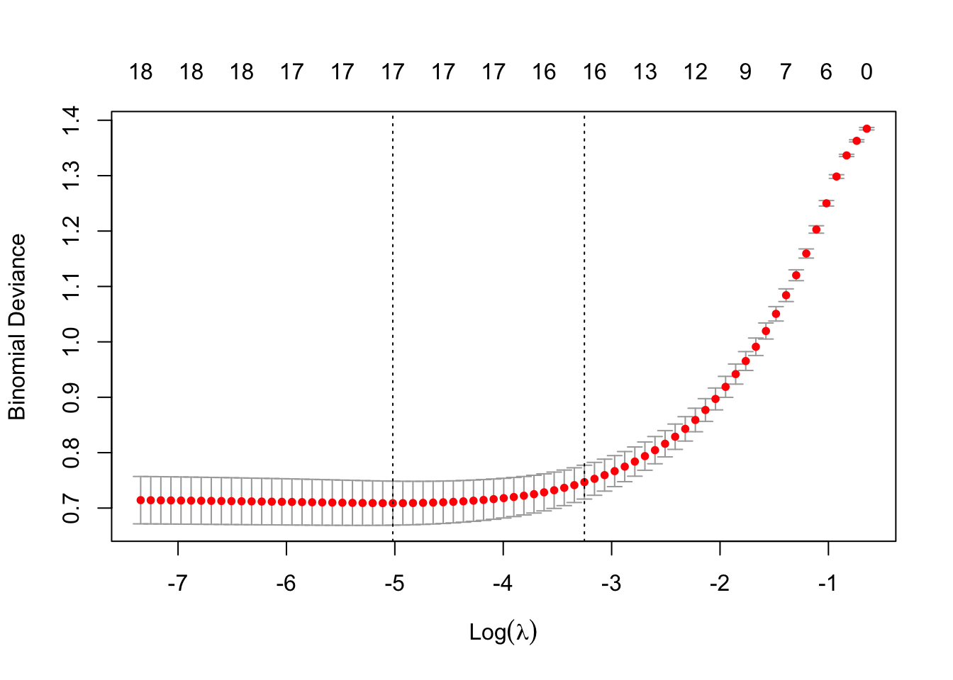
bestLambda <- cv_model$lambda.minThe plot shows how the model’s prediction error changes with different values of lambda, \(λ\). It helps to identify the largest \(λ\) we can choose before the penalty starts to hurt performance - too much shrinkage can remove important predictors, increasing prediction error.
bestLambda[1] 0.006612261log(bestLambda)[1] -5.01883Time to see how well our model performs. Let’s predict if a individual is likely to have heart disease using our model and our test set.
y_pred <- predict(EN_model, s = bestLambda, newx = modTest, type = 'class')Just like for the logistic regression model we can calculate the accuracy of the prediction by comparing it to y_test with confusionMatrix().
y_pred <- as.factor(y_pred)

caret::confusionMatrix(y_pred, y_test)
Confusion Matrix and Statistics
Reference
Prediction 0 1
0 110 18
1 34 138
Accuracy : 0.8267
95% CI : (0.779, 0.8678)
No Information Rate : 0.52
P-Value [Acc > NIR] : < 2e-16
Kappa : 0.6513
Mcnemar's Test P-Value : 0.03751
Sensitivity : 0.7639
Specificity : 0.8846
Pos Pred Value : 0.8594
Neg Pred Value : 0.8023
Prevalence : 0.4800
Detection Rate : 0.3667
Detection Prevalence : 0.4267
Balanced Accuracy : 0.8243
'Positive' Class : 0
Our model performs relatively well with a Balanced Accuracy of 0.84.
Just like with linear or logistic regression, we can pull out the coefficients (weights) from our model to asses which variable(s) are the most explanatory for heart disease. We use the function coef() for this.
coeffs <- coef(EN_model, s = bestLambda)

coeffs
19 x 1 sparse Matrix of class "dgCMatrix"
s0
(Intercept) -0.2259971
age .
sex0 0.6333310
sex1 -0.5997203
chestPainType1 0.4142241
chestPainType2 1.4904347
chestPainType3 1.4408866
restBP -0.1945918
chol -0.1831287
fastingBP1 0.1874486
restElecCardio1 0.7630516
maxHR 0.4236329
exerciseAngina1 -0.6756953
STdepEKG -0.6492572
slopePeakExST1 -0.4919018
slopePeakExST2 0.1663786
nMajorVessels -0.9003091
DefectType2 0.3586529
DefectType3 -1.0024820First of all we see that none of our explanatory variables have been penalized so much that they have been removed, although some like age contribute very little to the model.
Let’s order the coefficients by size and plot them to get an easy overview. First we do a little data wrangling to set up the dataset.
coeffsDat <- as.data.frame(as.matrix(coeffs)) %>%
  rownames_to_column(var = 'VarName') %>%
  arrange(desc(s0)) %>%
  filter(!str_detect(VarName,"(Intercept)")) %>%
  mutate(VarName = factor(VarName, levels=VarName))
Now we can make a bar plot to visualize our results.
# Plot
ggplot(coeffsDat, aes(x = VarName, y = s0)) +
  geom_bar(stat = "identity", fill = "#9395D3") +
  coord_flip() +
  labs(title = "Feature Importance for Elastic Net",
       x = "Features",
       y = "Absolute Coefficients") +
  theme_classic()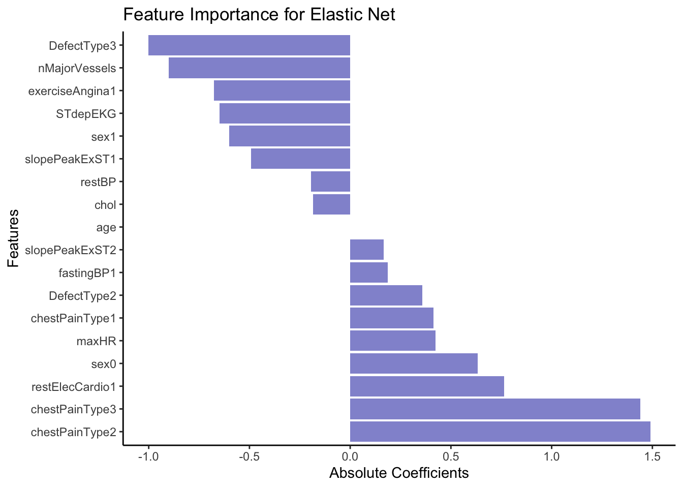
From the coefficients above it seem like cheat pain of any type (0 vs 1, 2 or 3) is a strong predictor of the outcome, e.g. heart disease. In opposition, having a DefectType3 significantly lowers the predicted probability of belonging to the event class (1 = Heart Disease). Specifically, it decreases the log-odds of belonging to class 1.
In terms of comparing the outcome of the Random Forest model with the Elastic Net Regression, don’t expect identical top features — they reflect different model assumptions.
Use both models as complementary tools:
EN: for interpretable, linear relationships
RF: for capturing complex patterns and variable interactions
If a feature ranks high in both models, it’s a strong signal that the feature is important.
If a feature ranks high in one but not the other — explore further: interaction? non-linearity? collinearity?