library(tidyverse)
library(ggplot2)
library(ContaminatedMixt)
library(factoextra)Presentation 5B: Kmeans and Random Forest
Part 1: K-means Clustering
Clustering is a type of unsupervised learning technique used to group similar data points together based on their features. The goal is to find inherent patterns or structures within the data, e.g. to see whether the data points fall into distinct groups with distinct features or not.
Wine dataset
For this we will use the wine data set as an example:
Let’s load in the dataset
data('wine') #load dataset
df_wine <- wine %>%
  as_tibble() #convert to tibble

df_wine
# A tibble: 178 × 14
Type Alcohol Malic Ash Alcalinity Magnesium Phenols Flavanoids
<fct> <dbl> <dbl> <dbl> <dbl> <int> <dbl> <dbl>
1 Barolo 14.2 1.71 2.43 15.6 127 2.8 3.06
2 Barolo 13.2 1.78 2.14 11.2 100 2.65 2.76
3 Barolo 13.2 2.36 2.67 18.6 101 2.8 3.24
4 Barolo 14.4 1.95 2.5 16.8 113 3.85 3.49
5 Barolo 13.2 2.59 2.87 21 118 2.8 2.69
6 Barolo 14.2 1.76 2.45 15.2 112 3.27 3.39
7 Barolo 14.4 1.87 2.45 14.6 96 2.5 2.52
8 Barolo 14.1 2.15 2.61 17.6 121 2.6 2.51
9 Barolo 14.8 1.64 2.17 14 97 2.8 2.98
10 Barolo 13.9 1.35 2.27 16 98 2.98 3.15
# ℹ 168 more rows
# ℹ 6 more variables: Nonflavanoid <dbl>, Proanthocyanins <dbl>, Color <dbl>,
# Hue <dbl>, Dilution <dbl>, Proline <int>This dataset contains 178 rows, each corresponding to one of three different cultivars of wine. It has 13 numerical columns that record different features of the wine.
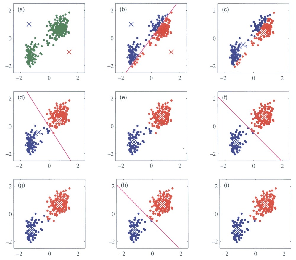
We will try out a popular method, k-means clustering. It works by initializing K centroids and assigning each data point to the nearest centroid. The algorithm then recalculates the centroids as the mean of the points in each cluster, repeating the process until the clusters stabilize. You can see an illustration of the process below. Its weakness is that we need to define the number of centroids, i.e. clusters, beforehand.
Running k-means
For k-means it is very important that the data is numeric and scaled so we will do that before running the algorithm.
# Set seed to ensure reproducibility
set.seed(123)

# Pull numeric variables and scale these
kmeans_df <- df_wine %>%
  dplyr::select(where(is.numeric)) %>%
  mutate(across(everything(), scale))

kmeans_df
# A tibble: 178 × 13
Alcohol[,1] Malic[,1] Ash[,1] Alcalinity[,1] Magnesium[,1] Phenols[,1]
<dbl> <dbl> <dbl> <dbl> <dbl> <dbl>
1 1.51 -0.561 0.231 -1.17 1.91 0.807
2 0.246 -0.498 -0.826 -2.48 0.0181 0.567
3 0.196 0.0212 1.11 -0.268 0.0881 0.807
4 1.69 -0.346 0.487 -0.807 0.928 2.48
5 0.295 0.227 1.84 0.451 1.28 0.807
6 1.48 -0.516 0.304 -1.29 0.858 1.56
7 1.71 -0.417 0.304 -1.47 -0.262 0.327
8 1.30 -0.167 0.888 -0.567 1.49 0.487
9 2.25 -0.623 -0.716 -1.65 -0.192 0.807
10 1.06 -0.883 -0.352 -1.05 -0.122 1.09
# ℹ 168 more rows
# ℹ 7 more variables: Flavanoids <dbl[,1]>, Nonflavanoid <dbl[,1]>,
# Proanthocyanins <dbl[,1]>, Color <dbl[,1]>, Hue <dbl[,1]>,
# Dilution <dbl[,1]>, Proline <dbl[,1]>K-means clustering in R is easy, we simply run the kmeans() function:
set.seed(123)

kmeans_res <- kmeans_df %>%
  kmeans(centers = 4, nstart = 25)

kmeans_res
K-means clustering with 4 clusters of sizes 45, 56, 49, 28
Cluster means:
Alcohol Malic Ash Alcalinity Magnesium Phenols
1 -0.9051690 -0.53898599 -0.6498944 0.1592193 -0.71473842 -0.4537841
2 0.9580555 -0.37748461 0.1969019 -0.8214121 0.39943022 0.9000233
3 0.1860184 0.90242582 0.2485092 0.5820616 -0.05049296 -0.9857762
4 -0.7869073 0.04195151 0.2157781 0.3683284 0.43818899 0.6543578
Flavanoids Nonflavanoid Proanthocyanins Color Hue Dilution
1 -0.2408779 0.3315072 -0.4329238 -0.9177666 0.5202140 0.07869143
2 0.9848901 -0.6204018 0.5575193 0.2423047 0.4799084 0.76926636
3 -1.2327174 0.7148253 -0.7474990 0.9857177 -1.1879477 -1.29787850
4 0.5746004 -0.5429201 0.8888549 -0.7346332 0.2830335 0.60628629
Proline
1 -0.7820425
2 1.2184972
3 -0.3789756
4 -0.5169332
Clustering vector:
[1] 2 2 2 2 4 2 2 2 2 2 2 2 2 2 2 2 2 2 2 2 2 4 2 2 2 4 2 2 2 2 2 2 2 2 2 2 2
[38] 2 2 2 2 2 2 4 2 2 2 2 2 2 2 2 2 2 2 2 2 2 2 1 1 1 1 4 1 4 2 1 1 4 1 4 1 4
[75] 4 1 1 1 4 4 1 1 1 3 4 1 1 1 1 1 1 1 1 4 4 4 4 1 4 4 1 1 4 1 1 1 1 1 1 4 4
[112] 1 1 1 1 1 1 1 1 1 4 4 4 4 4 1 4 1 1 1 3 3 3 3 3 3 3 3 3 3 3 3 3 3 3 3 3 3
[149] 3 3 3 3 3 3 3 3 3 3 3 3 3 3 3 3 3 3 3 3 3 3 3 3 3 3 3 3 3 3
Within cluster sum of squares by cluster:
[1] 289.9515 268.5747 302.9915 307.0966
(between_SS / total_SS = 49.2 %)
Available components:
[1] "cluster" "centers" "totss" "withinss" "tot.withinss"
[6] "betweenss" "size" "iter" "ifault" We can call kmeans_res$centers to inspect the values of the centroids. For example the center of cluster 1 is placed at the coordinates -0.79 for Alcohol, 0.04 for Malic Acid, 0.22 for Ash and so on. Since our data has 13 dimensions, i.e. features, the cluster centers also do.
This is not super practical if we would like to visually inspect the clustering since we cannot plot in 13 dimensions. How could we solve this?
Visualizing k-means results
We would like to see where our wine bottles and their clusters lie in a low-dimensional space. This can easily be done using the fviz_cluster()
fviz_cluster(object = kmeans_res,
             data = kmeans_df,
             palette = c("#2E9FDF", "#00AFBB", "#E7B800", "orchid3"),
             geom = "point",
             ellipse.type = "norm",
             ggtheme = theme_bw())
Optimal number of clusters
There are several ways to investigate the ideal number of clusters and fviz_nbclust from the factoextra package provides three of them:
The so-called elbow method observes how the sum of squared errors (sse) changes as we vary the number of clusters. This is also sometimes referred to as “within sum of square” (wss).
kmeans_df %>%
  fviz_nbclust(kmeans, method = "wss")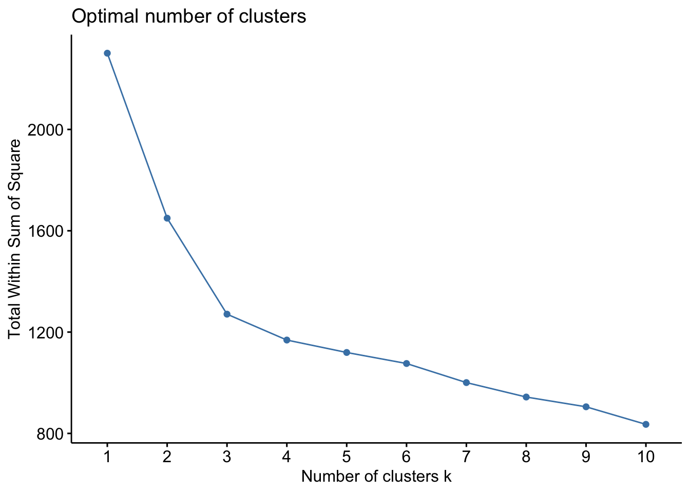
The gap statistic compares the within-cluster variation (how compact the clusters are) for different values of K to the expected variation under a null reference distribution (i.e., random clustering).
kmeans_df %>%
  fviz_nbclust(kmeans, method = "gap_stat")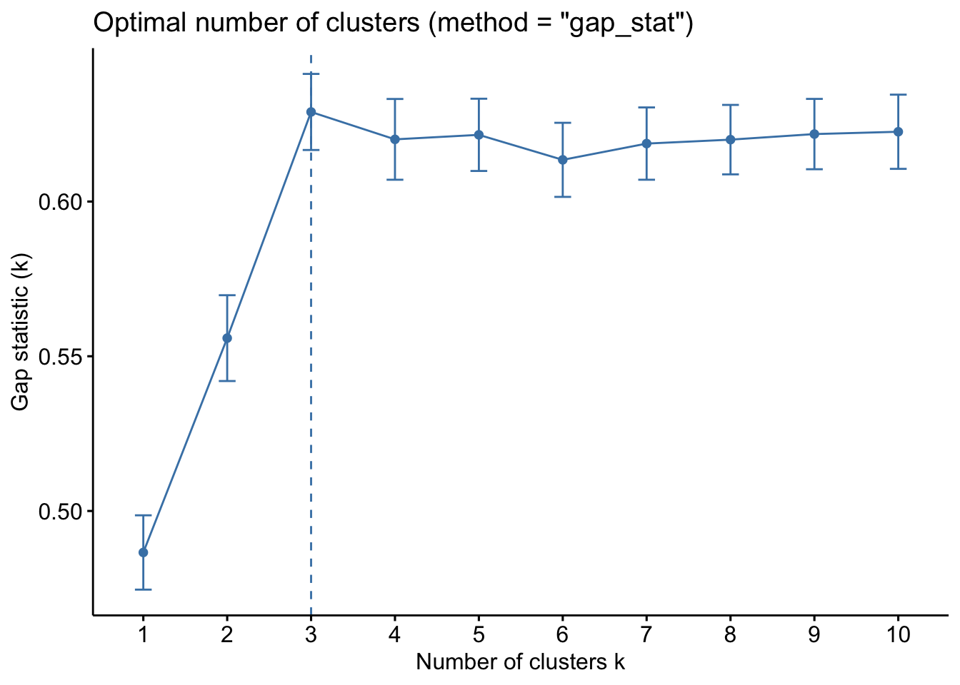
Both of these tell us that there should be three clusters and we also know that there are three cultivars of wine in the dataset. Let’s redo k-means with three centroids.
# Set seed to ensure reproducibility
set.seed(123)

#run kmeans
kmeans_res <- kmeans_df %>%
  kmeans(centers = 3, nstart = 25)
#add updated cluster info to the dataframe
fviz_cluster(kmeans_res, data = kmeans_df,
palette = c("#2E9FDF", "#00AFBB", "#E7B800"),
geom = "point",
ellipse.type = "norm",
ggtheme = theme_bw())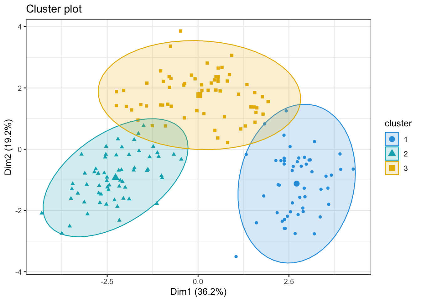
Now, some obvious questions to ask might be (I) how do the clusters relate to the three cultivars of wine in the dataset? and (II) which variables are mainly driving the clustering?
Question (I) can be can be answered somewhat easily simply by coloring the clusters according to wine label or adding the label to the points in the plot above.
fzPlot <- fviz_cluster(kmeans_res, data = kmeans_df,
             palette = c("#2E9FDF", "#00AFBB", "#E7B800"),
             geom = "point",
             ellipse.type = "norm",
             ggtheme = theme_bw())


wine_labs <- transform(fzPlot$data,
                       my_label = df_wine$Type)

wine_labs
name x y coord cluster my_label
1 1 -3.30742097 -1.43940225 13.0109123 2 Barolo
2 2 -2.20324981 0.33245507 4.9648361 2 Barolo
3 3 -2.50966069 -1.02825072 7.3556964 2 Barolo
4 4 -3.74649719 -2.74861839 21.5911443 2 Barolo
5 5 -1.00607049 -0.86738404 1.7645329 2 Barolo
6 6 -3.04167373 -2.11643092 13.7310589 2 Barolo
7 7 -2.44220051 -1.17154534 7.3368618 2 Barolo
8 8 -2.05364379 -1.60443714 6.7916714 2 Barolo
9 9 -2.50381135 -0.91548847 7.1071904 2 Barolo
10 10 -2.74588238 -0.78721703 8.1595807 2 Barolo
11 11 -3.46994837 -1.29866985 13.7270851 2 Barolo
12 12 -1.74981688 -0.61025577 3.4342712 2 Barolo
13 13 -2.10751729 -0.67380561 4.8956431 2 Barolo
14 14 -3.44842921 -1.12744948 13.1628064 2 Barolo
15 15 -4.30065228 -2.09007971 22.8640433 2 Barolo
16 16 -2.29870383 -1.65787506 8.0325890 2 Barolo
17 17 -2.16584568 -2.32075875 10.0768087 2 Barolo
18 18 -1.89362947 -1.62677993 6.2322455 2 Barolo
19 19 -3.53202167 -2.51125971 18.7816024 2 Barolo
20 20 -2.07865856 -1.05815307 5.4405093 2 Barolo
21 21 -3.11561376 -0.78468361 10.3227775 2 Barolo
22 22 -1.08351361 -0.24106354 1.2321134 2 Barolo
23 23 -2.52809263 0.09158228 6.3996397 2 Barolo
24 24 -1.64036108 0.51482667 2.9558310 2 Barolo
25 25 -1.75662066 0.31625681 3.1857345 2 Barolo
26 26 -0.98729406 -0.93802129 1.8546335 2 Barolo
27 27 -1.77028387 -0.68424496 3.6020961 2 Barolo
28 28 -1.23194878 0.08955442 1.5257178 2 Barolo
29 29 -2.18225047 -0.68762990 5.2350520 2 Barolo
30 30 -2.24976267 -0.19092336 5.0978838 2 Barolo
31 31 -2.49318704 -1.23734344 7.7470004 2 Barolo
32 32 -2.66987964 -1.46773335 9.2824985 2 Barolo
33 33 -1.62399801 -0.05255620 2.6401317 2 Barolo
34 34 -1.89733870 -1.62846673 6.2517980 2 Barolo
35 35 -1.40642118 -0.69597107 2.4623963 2 Barolo
36 36 -1.89847087 -0.17621387 3.6352430 2 Barolo
37 37 -1.38096669 -0.65678714 2.3384383 2 Barolo
38 38 -1.11905070 -0.11378878 1.2652224 2 Barolo
39 39 -1.49796891 0.76726764 2.8326105 2 Barolo
40 40 -2.52268490 -1.79793023 9.5964922 2 Barolo
41 41 -2.58081526 -0.77742329 7.2649943 2 Barolo
42 42 -0.66660159 -0.16948285 0.4730821 2 Barolo
43 43 -3.06216898 -1.15266742 10.7055210 2 Barolo
44 44 -0.46090897 -0.32981177 0.3212129 2 Barolo
45 45 -2.09544094 0.07080918 4.3958867 2 Barolo
46 46 -1.13297020 -1.77210849 4.4239900 2 Barolo
47 47 -2.71893118 -1.18798353 8.8038917 2 Barolo
48 48 -2.81340300 -0.64444071 8.3305403 2 Barolo
49 49 -2.00419725 -1.24352164 5.5631527 2 Barolo
50 50 -2.69987528 -1.74703922 10.3414726 2 Barolo
51 51 -3.20587409 -0.16652226 10.3053583 2 Barolo
52 52 -2.85091773 -0.74318238 8.6800519 2 Barolo
53 53 -3.49574328 -1.60819732 14.8065197 2 Barolo
54 54 -2.21853316 -1.86989325 8.4183902 2 Barolo
55 55 -2.14094846 -1.01389147 5.6116362 2 Barolo
56 56 -2.46238340 -1.32526988 7.8196723 2 Barolo
57 57 -2.73380617 -1.43250785 9.5257749 2 Barolo
58 58 -2.16762631 -1.20878999 6.1597770 2 Barolo
59 59 -3.13054925 -1.72670828 12.7818601 2 Barolo
60 60 0.92596992 3.06484062 10.2506683 3 Grignolino
61 61 1.53814123 1.37755758 4.2635433 3 Grignolino
62 62 1.83108449 0.82764942 4.0378740 1 Grignolino
63 63 -0.03052074 1.25923400 1.5866018 3 Grignolino
64 64 -2.04449433 1.91961759 7.8648888 3 Grignolino
65 65 0.60796583 1.90269154 3.9898575 3 Grignolino
66 66 -0.89769555 0.76176263 1.3861396 3 Grignolino
67 67 -2.24218226 1.87929123 8.5591168 3 Grignolino
68 68 -0.18286818 2.42031869 5.8913833 3 Grignolino
69 69 0.81051865 0.21989369 0.7052937 3 Grignolino
70 70 -1.97006319 1.39933587 5.8392898 3 Grignolino
71 71 1.56779366 0.88249373 3.2367721 3 Grignolino
72 72 -1.65301884 0.95402102 3.6426274 3 Grignolino
73 73 0.72333196 1.06065342 1.6481948 3 Grignolino
74 74 -2.55501977 -0.25946663 6.5954489 2 Grignolino
75 75 -1.82741266 1.28425547 4.9887491 3 Grignolino
76 76 0.86555129 2.43722606 6.6892499 3 Grignolino
77 77 -0.36897357 2.14784815 4.7493932 3 Grignolino
78 78 1.45327752 1.37946048 4.0149268 3 Grignolino
79 79 -1.25937829 0.76868117 2.1769044 3 Grignolino
80 80 -0.37509228 1.02415439 1.1895864 3 Grignolino
81 81 -0.75992026 3.36555997 11.9044727 3 Grignolino
82 82 -1.03166776 1.44662897 3.1570737 3 Grignolino
83 83 0.49348469 2.37454522 5.8819921 3 Grignolino
84 84 2.53183508 0.08719738 6.4177923 1 Grignolino
85 85 -0.83297044 1.46952520 2.8533441 3 Grignolino
86 86 -0.78568828 2.02092573 4.7014469 3 Grignolino
87 87 0.80456258 2.22754675 5.6092855 3 Grignolino
88 88 0.55647288 2.36631035 5.9090867 3 Grignolino
89 89 1.11197430 1.79717757 4.4663340 3 Grignolino
90 90 0.55415961 2.65006452 7.3299348 3 Grignolino
91 91 1.34548982 2.11204365 6.2710712 3 Grignolino
92 92 1.56008180 1.84700434 5.8452803 3 Grignolino
93 93 1.92711944 1.55510868 6.1321523 3 Grignolino
94 94 -0.74456561 2.30642556 5.8739768 3 Grignolino
95 95 -0.95476209 2.21727377 5.8278736 3 Grignolino
96 96 -2.53670943 -0.16879786 6.4633875 2 Grignolino
97 97 0.54242248 0.36788878 0.4295643 3 Grignolino
98 98 -1.02814946 2.55835254 7.6022591 3 Grignolino
99 99 -2.24557492 1.42871116 7.0838223 3 Grignolino
100 100 -1.40624916 2.16009839 6.6435617 3 Grignolino
101 101 -0.79547585 2.37026258 6.2509265 3 Grignolino
102 102 0.54798592 2.28667820 5.5291858 3 Grignolino
103 103 0.16072037 1.16120769 1.3742343 3 Grignolino
104 104 0.65793897 2.67242260 7.5747263 3 Grignolino
105 105 -0.39125074 2.09282809 4.5330066 3 Grignolino
106 106 1.76751314 1.71245783 6.0566145 3 Grignolino
107 107 0.36523707 2.16325103 4.8130531 3 Grignolino
108 108 1.61611371 1.35177021 4.4391062 3 Grignolino
109 109 -0.08230361 2.29974728 5.2956114 3 Grignolino
110 110 -1.57383547 1.45792167 4.6024937 3 Grignolino
111 111 -1.41657326 1.41421730 4.0066904 3 Grignolino
112 112 0.27791878 1.92513751 3.7833933 3 Grignolino
113 113 1.29947929 0.76102555 2.2678063 3 Grignolino
114 114 0.45578615 2.26303187 5.3290542 3 Grignolino
115 115 0.49279573 1.93359062 3.9816203 3 Grignolino
116 116 -0.48071836 3.86089273 15.1375828 3 Grignolino
117 117 0.25217752 2.81355567 7.9796890 3 Grignolino
118 118 0.10692601 1.92349609 3.7112704 3 Grignolino
119 119 2.42616867 1.25360477 7.4578193 1 Grignolino
120 120 0.54953935 2.21591073 5.2122539 3 Grignolino
121 121 -0.73754141 1.40499335 2.5179736 3 Grignolino
122 122 -1.33256273 -0.25262431 1.8395425 2 Grignolino
123 123 1.17377592 0.66209914 1.8161252 3 Grignolino
124 124 0.46103449 0.61654897 0.5926854 3 Grignolino
125 125 -0.97572169 1.44150419 3.0299671 3 Grignolino
126 126 0.09653741 2.10406268 4.4363993 3 Grignolino
127 127 -0.03837888 1.26319878 1.5971441 3 Grignolino
128 128 1.59266578 1.20474513 3.9879951 3 Grignolino
129 129 0.47821593 1.93338681 3.9666750 3 Grignolino
130 130 1.78779033 1.14705241 4.5119235 3 Grignolino
131 131 1.32336859 -0.16990994 1.7801738 1 Barbera
132 132 2.37779336 -0.37352893 5.7934251 1 Barbera
133 133 2.92867865 -0.26311960 8.6463906 1 Barbera
134 134 2.14077227 -0.36721907 4.7177558 1 Barbera
135 135 2.36320318 0.45834188 5.7948065 1 Barbera
136 136 3.05522315 -0.35241870 9.4585874 1 Barbera
137 137 3.90473898 -0.15414769 15.2707480 1 Barbera
138 138 3.92539034 -0.65783157 15.8414317 1 Barbera
139 139 3.08557209 -0.34786148 9.6417627 1 Barbera
140 140 2.36779237 -0.29115903 5.6912143 1 Barbera
141 141 2.77099630 -0.28599811 7.7602154 1 Barbera
142 142 2.28012931 -0.37146000 5.3369722 1 Barbera
143 143 2.97723506 -0.48784177 9.1019182 1 Barbera
144 144 2.36851341 -0.48097694 5.8411946 1 Barbera
145 145 2.20364930 -1.15678934 6.1942318 1 Barbera
146 146 2.61823528 -0.56157662 7.1705243 1 Barbera
147 147 4.26859758 -0.64784348 18.6406264 1 Barbera
148 148 3.57256360 -1.26912271 14.3738831 1 Barbera
149 149 2.79916760 -1.56611596 10.2880585 1 Barbera
150 150 2.89150275 -2.03531563 12.5032979 1 Barbera
151 151 2.31420887 -2.34973775 10.8768302 1 Barbera
152 152 2.54265841 -2.03952982 10.6247937 1 Barbera
153 153 1.80744271 -1.52334876 5.5874406 1 Barbera
154 154 2.75238051 -2.13291565 12.1249276 1 Barbera
155 155 2.72945105 -0.40873328 7.6169659 1 Barbera
156 156 3.59472857 -1.79731421 16.1524119 1 Barbera
157 157 2.88169708 -1.91980308 11.9898219 1 Barbera
158 158 3.38261413 -1.30818615 13.1534293 1 Barbera
159 159 1.04523342 -3.50520194 13.3789535 1 Barbera
160 160 1.60538369 -2.39986842 8.3366252 1 Barbera
161 161 3.13428951 -0.73608464 10.3655913 1 Barbera
162 162 2.23385546 -1.17215877 6.3640664 1 Barbera
163 163 2.83966343 -0.55447984 8.3711363 1 Barbera
164 164 2.59019044 -0.69600220 7.1935056 1 Barbera
165 165 2.94100316 -1.55093397 11.0548957 1 Barbera
166 166 3.52010248 -0.88004430 13.1655994 1 Barbera
167 167 2.39934228 -2.58506402 12.4393994 1 Barbera
168 168 2.92084537 -1.27086200 10.1464279 1 Barbera
169 169 2.17527658 -2.07169331 9.0237414 1 Barbera
170 170 2.37423037 -2.58138565 12.3005217 1 Barbera
171 171 3.20258311 0.25054235 10.3193101 1 Barbera
172 172 3.66757294 -0.84536318 14.1657302 1 Barbera
173 173 2.45862032 -2.18762727 10.8305270 1 Barbera
174 174 3.36104305 -2.21005484 16.1809528 1 Barbera
175 175 2.59463669 -1.75228636 9.8026471 1 Barbera
176 176 2.67030685 -2.75313287 14.7102793 1 Barbera
177 177 2.38030254 -2.29088437 10.9139914 1 Barbera
178 178 3.19973210 -2.76113075 17.8621285 1 BarberafzPlot + geom_text(data = wine_labs,
aes(label = my_label), size = 2.5)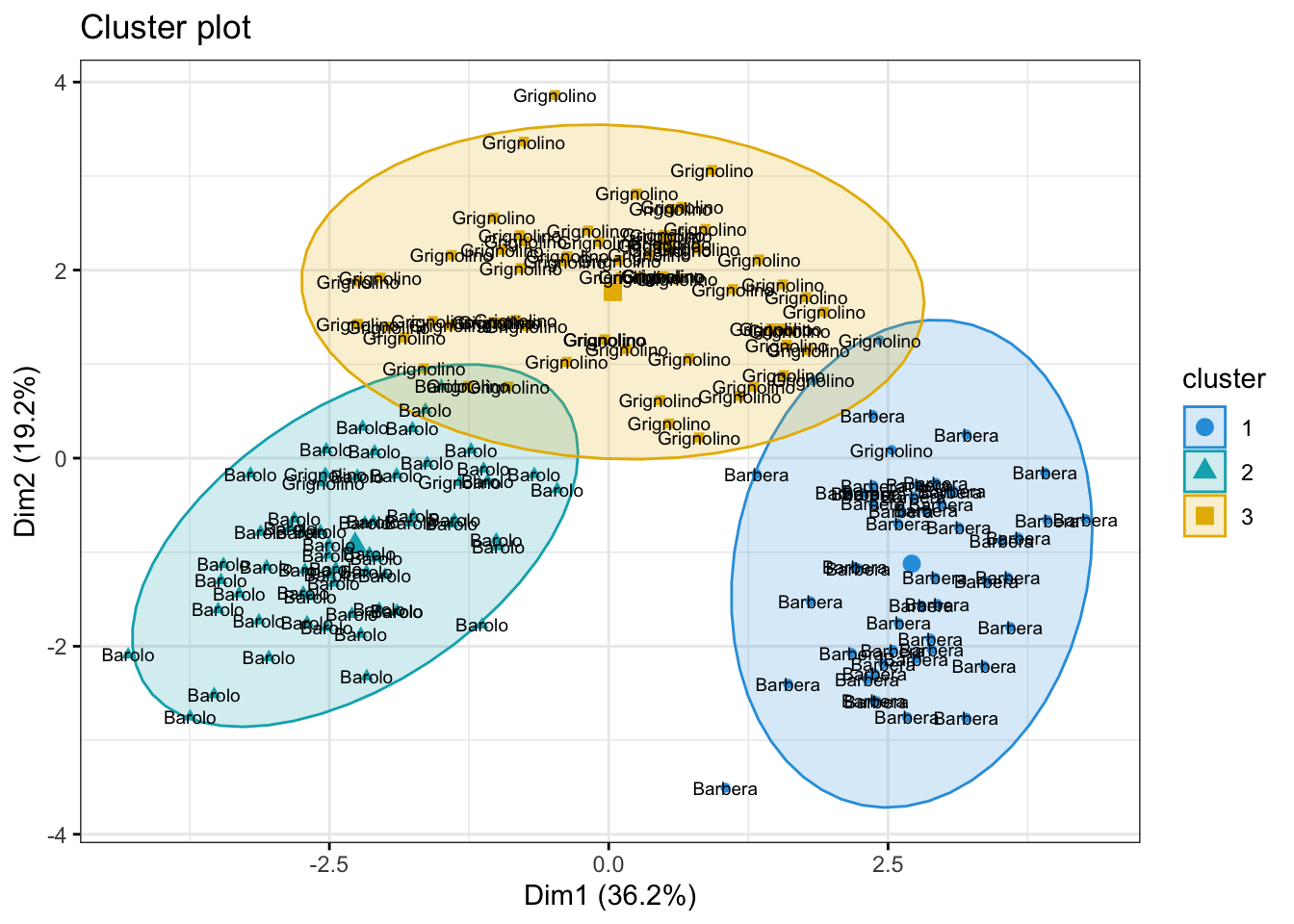
The answer to question (II) is a bit more tricky. One way to get a sense of which variables may be contributing to the clustering is to examine the variance of the cluster centers for each variable. A higher variance suggests that the cluster centroids differ more on that variable, so that variable may be playing a larger role in separating the clusters.
Note: This is only a descriptive heuristic, not a statistical test. Unlike PCA, k-means does not produce loadings, so there is no direct measure of variable importance in the same sense.
kmeans_res$centers Alcohol Malic Ash Alcalinity Magnesium Phenols
1 0.1644436 0.8690954 0.1863726 0.5228924 -0.07526047 -0.97657548
2 0.8328826 -0.3029551 0.3636801 -0.6084749 0.57596208 0.88274724
3 -0.9234669 -0.3929331 -0.4931257 0.1701220 -0.49032869 -0.07576891
Flavanoids Nonflavanoid Proanthocyanins Color Hue Dilution
1 -1.21182921 0.72402116 -0.77751312 0.9388902 -1.1615122 -1.2887761
2 0.97506900 -0.56050853 0.57865427 0.1705823 0.4726504 0.7770551
3 0.02075402 -0.03343924 0.05810161 -0.8993770 0.4605046 0.2700025
Proline
1 -0.4059428
2 1.1220202
3 -0.7517257var_importance <- apply(kmeans_res$centers, 2, var)
sort(var_importance, decreasing = TRUE) Flavanoids Dilution Proline Hue Phenols
1.2020837 1.1590920 0.9941934 0.8835955 0.8645478
Color Alcohol Malic Proanthocyanins Nonflavanoid
0.8523894 0.7858539 0.4957524 0.4680695 0.4169275
Alcalinity Magnesium Ash
0.3351087 0.2888914 0.2045454 Part 2: Random Forest
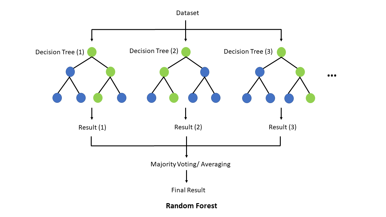
In this section, we will train a Random Forest (RF) model. Random Forest is a simple ensemble machine learning method that builds multiple decision trees and combines their predictions to improve accuracy and robustness. By averaging the results of many trees, it reduces overfitting and increases generalization, making it particularly effective for complex, non-linear relationships. One of its key strengths is its ability to handle large datasets with many features, while also providing insights into feature importance.
Why do we want to try a RF? Unlike linear, logistic, or elastic net regression (presentation 5C - only if time permits), RF does not require predictors (or model residuals) to be normally distributed, nor does RF assume a linear relationship between predictors and the outcome — it can naturally capture non-linear patterns and complex interactions between variables.
Another advantage is that RF considers one predictor at a time when splitting at a predictor, making it robust to differences in variable scales and allowing it to handle categorical variables directly.
The downside to a is RF model is that it typically require a reasonably large sample size to perform well and can be less interpretable compared to regression-based approaches.
First and foremost, lets load the R packages needed for analysis:
library(tidyverse)
library(caret)
library(randomForest)
For this exercise we will use a dataset from patients with Heart Disease. Information on the columns in the dataset can be found here.
HD <- read_csv("../data/HeartDisease.csv")

head(HD)
# A tibble: 6 × 14
age sex chestPainType restBP chol fastingBP restElecCardio maxHR
<dbl> <dbl> <dbl> <dbl> <dbl> <dbl> <dbl> <dbl>
1 52 1 0 125 212 0 1 168
2 53 1 0 140 203 1 0 155
3 70 1 0 145 174 0 1 125
4 61 1 0 148 203 0 1 161
5 62 0 0 138 294 1 1 106
6 58 0 0 100 248 0 0 122
# ℹ 6 more variables: exerciseAngina <dbl>, STdepEKG <dbl>,
# slopePeakExST <dbl>, nMajorVessels <dbl>, DefectType <dbl>,
# heartDisease <dbl>table(HD$chestPainType)
  0   1   2   3
497 167 284  77
Let’s convert some of the variables that are encoded as numeric datatypes but should be factors:
facCols <- c("sex",
             "chestPainType",
             "fastingBP",
             "restElecCardio",
             "exerciseAngina",
             "slopePeakExST",
             "DefectType",
             "heartDisease")

HD <- HD %>%
  mutate(across(all_of(facCols), as.factor))


head(HD)
# A tibble: 6 × 14
age sex chestPainType restBP chol fastingBP restElecCardio maxHR
<dbl> <fct> <fct> <dbl> <dbl> <fct> <fct> <dbl>
1 52 1 0 125 212 0 1 168
2 53 1 0 140 203 1 0 155
3 70 1 0 145 174 0 1 125
4 61 1 0 148 203 0 1 161
5 62 0 0 138 294 1 1 106
6 58 0 0 100 248 0 0 122
# ℹ 6 more variables: exerciseAngina <fct>, STdepEKG <dbl>,
# slopePeakExST <fct>, nMajorVessels <dbl>, DefectType <fct>,
# heartDisease <fct>Next, let’s do some summary statistics to have a look at the variables we have in our dataset. Firstly, the numeric columns. We can get a quick overview of variable distributions and ranges with some histograms.
# Reshape data to long format for ggplot2
long_data <- HD %>%
  dplyr::select(where(is.numeric)) %>%
  pivot_longer(cols = everything(),
               names_to = "variable",
               values_to = "value")

head(long_data)
# A tibble: 6 × 2
variable value
<chr> <dbl>
1 age 52
2 restBP 125
3 chol 212
4 maxHR 168
5 STdepEKG 1
6 nMajorVessels 2# Plot histograms for each numeric variable in one grid
ggplot(long_data,
aes(x = value)) +
geom_histogram(binwidth = 0.5, fill = "#9395D3", color ='grey30') +
facet_wrap(vars(variable), scales = "free") +
theme_minimal()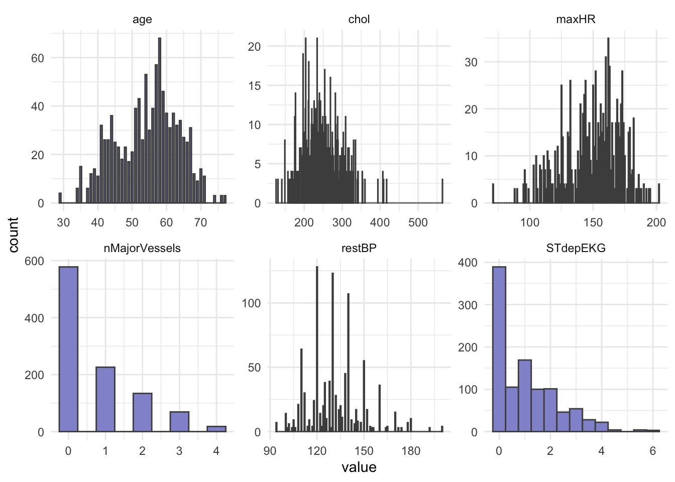
Importantly, let’s check the balance of the categorical/factor variables.
HD %>%
  dplyr::select(where(is.factor)) %>%
  pivot_longer(everything(), names_to = "Variable", values_to = "Level") %>%
  dplyr::count(Variable, Level, name = "Count")
# A tibble: 22 × 3
Variable Level Count
<chr> <fct> <int>
1 DefectType 0 7
2 DefectType 1 64
3 DefectType 2 544
4 DefectType 3 410
5 chestPainType 0 497
6 chestPainType 1 167
7 chestPainType 2 284
8 chestPainType 3 77
9 exerciseAngina 0 680
10 exerciseAngina 1 345
# ℹ 12 more rows# OR
# cat_cols <- HD_EN %>% dplyr::select(where(is.factor)) %>% colnames()
#
# for (col in cat_cols){
# print(col)
# print(table(HD_EN[[col]]))
# }From our count table above we see that variables DefectType, chestPainType, restElecCardio, and slopePeakExST are unbalanced. Especially DefectType and restElecCardio are problematic with only 7 and 15 observations for one of the factor levels.
To avoid issues when modelling, we will filter out these observations and re-level the two variables.
HD_RF <- HD %>%
  filter(DefectType != "0", restElecCardio != "2") %>%
  mutate(DefectType = as.factor(as.character(DefectType)),
         restElecCardio = as.factor(as.character(restElecCardio)))
head(HD_RF)
# A tibble: 6 × 14
age sex chestPainType restBP chol fastingBP restElecCardio maxHR
<dbl> <fct> <fct> <dbl> <dbl> <fct> <fct> <dbl>
1 52 1 0 125 212 0 1 168
2 53 1 0 140 203 1 0 155
3 70 1 0 145 174 0 1 125
4 61 1 0 148 203 0 1 161
5 62 0 0 138 294 1 1 106
6 58 0 0 100 248 0 0 122
# ℹ 6 more variables: exerciseAngina <fct>, STdepEKG <dbl>,
# slopePeakExST <fct>, nMajorVessels <dbl>, DefectType <fct>,
# heartDisease <fct>In addition to ensuring an at least somewhat balanced data set, RF requires the outcome variable to be a categorical type, meaning we must convert heartDisease from a binary (0 or 1) variables to a category variable.
# Mutate outcome to category and add ID column for splitting
HD_RF <- HD_RF %>%
  mutate(heartDisease = fct_recode(heartDisease, noHD = "0", yesHD = "1"))

head(HD_RF$heartDisease)
[1] noHD noHD noHD noHD noHD yesHD
Levels: noHD yesHDTrain & Test Set
We split our dataset into train and test set, we will keep 70% of the data in the training set and take out 30% for the test set. Importantly, we must ensure that all levels of each categorical/factor variable are represented in both sets! There are different ways of doing this in R, but one very easy way to achieve a good split is with the createDataPartition() function from caret.
# Set seed to ensure same split when code is re-run
set.seed(123)

#
idx <- createDataPartition(HD_RF$heartDisease, p = 0.7, list = FALSE)
train <- HD_RF[idx, ]
test  <- HD_RF[-idx, ]
# Split on outcome variable
table(train$heartDisease)
 noHD yesHD
339 364 table(test$heartDisease)
 noHD yesHD
  144   156
In our case, because we have a fairly balanced dataset, we are lucky and all levels of the outcome variable can be represented in both sets. If this was not the case, we might have had to remove some variables (or levels) altogether.
Random Forest Model
Now let’s set up a RF model with cross-validation - this way we do not overfit our model. The R-package caret has a very versatile function trainControl() which can be used with a range of re-sampling methods including bootstrapping, out-of-bag error, and leave-one-out cross-validation.
set.seed(123)

# Set up cross-validation: 5-fold CV
RFcv <- trainControl(
  method = "cv",
  number = 5,
  classProbs = TRUE,
  summaryFunction = twoClassSummary,
  savePredictions = "final"
)

RFcv
$method
[1] "cv"
$number
[1] 5
$repeats
[1] NA
$search
[1] "grid"
$p
[1] 0.75
$initialWindow
NULL
$horizon
[1] 1
$fixedWindow
[1] TRUE
$skip
[1] 0
$verboseIter
[1] FALSE
$returnData
[1] TRUE
$returnResamp
[1] "final"
$savePredictions
[1] "final"
$classProbs
[1] TRUE
$summaryFunction
function (data, lev = NULL, model = NULL)
{
if (length(lev) > 2) {
stop(paste("Your outcome has", length(lev), "levels. The twoClassSummary() function isn't appropriate."))
}
requireNamespaceQuietStop("pROC")
if (!all(levels(data[, "pred"]) == lev)) {
stop("levels of observed and predicted data do not match")
}
rocObject <- try(pROC::roc(data$obs, data[, lev[1]], direction = ">",
quiet = TRUE), silent = TRUE)
rocAUC <- if (inherits(rocObject, "try-error"))
NA
else rocObject$auc
out <- c(rocAUC, sensitivity(data[, "pred"], data[, "obs"],
lev[1]), specificity(data[, "pred"], data[, "obs"], lev[2]))
names(out) <- c("ROC", "Sens", "Spec")
out
}
<bytecode: 0x10f075c10>
<environment: namespace:caret>
$selectionFunction
[1] "best"
$preProcOptions
$preProcOptions$thresh
[1] 0.95
$preProcOptions$ICAcomp
[1] 3
$preProcOptions$k
[1] 5
$preProcOptions$freqCut
[1] 19
$preProcOptions$uniqueCut
[1] 10
$preProcOptions$cutoff
[1] 0.9
$sampling
NULL
$index
NULL
$indexOut
NULL
$indexFinal
NULL
$timingSamps
[1] 0
$predictionBounds
[1] FALSE FALSE
$seeds
[1] NA
$adaptive
$adaptive$min
[1] 5
$adaptive$alpha
[1] 0.05
$adaptive$method
[1] "gls"
$adaptive$complete
[1] TRUE
$trim
[1] FALSE
$allowParallel
[1] TRUENow that we have set up parameters for cross validation in the RFcv object above, we can feed it to the train() function from the caret packages. We also specify the training data, the name of the outcome variable, and, importantly, that we want to perform random forest (method = "rf") as the train() function can be used for different models.
set.seed(123)

rf_model <- train(
  x = train %>% dplyr::select(-heartDisease),
  y = train$heartDisease,
  method = "rf",
  trControl = RFcv,
  metric = "Accuracy",
  tuneLength = 5,
  importance = TRUE
)

print(rf_model)
Random Forest
703 samples
13 predictor
2 classes: 'noHD', 'yesHD'
No pre-processing
Resampling: Cross-Validated (5 fold)
Summary of sample sizes: 563, 562, 562, 563, 562
Resampling results across tuning parameters:
mtry ROC Sens Spec
2 0.9929161 0.9645742 0.9945205
4 0.9927587 0.9675154 0.9945205
7 0.9940726 0.9645303 0.9945205
10 0.9942133 0.9645303 0.9945205
13 0.9937031 0.9645303 0.9917808
ROC was used to select the optimal model using the largest value.
The final value used for the model was mtry = 10.Next, we can plot your model fit to see how many explanatory variables significantly contribute to our model.
# Best parameters
rf_model$bestTune
mtry
4 10# Plot performance
plot(rf_model)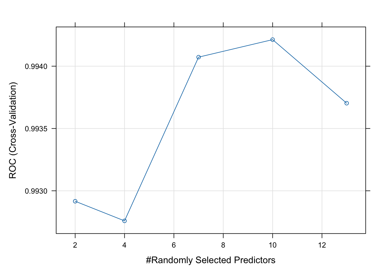
As we see from the plot above, the model performs best with four variables randomly sampled as candidates at each split (mtry = 10). There are different tuning parameters in a random forest, these include; n_estimators (number of trees), max_features (features to try at splits), max_depth (tree depth), and min_samples_split (minimum number of samples required to split a node).
The tuneLength argument in the train() function specifies how many different values of the tuning parameters to try.
Next, we use the test set to evaluate our model performance. We will do this with the predict function, which will give us the predicted probabilities for each class.
# Predict class probabilities
y_pred <- predict(rf_model, newdata = test, type = "prob")
head(y_pred)
noHD yesHD
1 0.994 0.006
2 0.968 0.032
3 0.016 0.984
4 1.000 0.000
5 0.998 0.002
6 1.000 0.000As the output of predict is a probability of belonging to a specific class, we will need to convert these probabilities to class labels (yesHD or noHD). This way we can compare a predicted label with the true label in the test set to evaluate our model performance.
y_pred <- as.factor(ifelse(y_pred$yesHD > 0.5, "yesHD", "noHD"))

caret::confusionMatrix(y_pred, test$heartDisease)
Confusion Matrix and Statistics
Reference
Prediction noHD yesHD
noHD 141 0
yesHD 3 156
Accuracy : 0.99
95% CI : (0.9711, 0.9979)
No Information Rate : 0.52
P-Value [Acc > NIR] : <2e-16
Kappa : 0.98
Mcnemar's Test P-Value : 0.2482
Sensitivity : 0.9792
Specificity : 1.0000
Pos Pred Value : 1.0000
Neg Pred Value : 0.9811
Prevalence : 0.4800
Detection Rate : 0.4700
Detection Prevalence : 0.4700
Balanced Accuracy : 0.9896
'Positive' Class : noHD
Lastly, we can extract the predictive variables with the greatest importance from your fit.
varImpOut <- varImp(rf_model)

varImpOut$importance
noHD yesHD
age 62.08613 62.08613
sex 30.02973 30.02973
chestPainType 94.83905 94.83905
restBP 65.98055 65.98055
chol 75.11579 75.11579
fastingBP 0.00000 0.00000
restElecCardio 20.85050 20.85050
maxHR 63.45448 63.45448
exerciseAngina 12.77844 12.77844
STdepEKG 93.18319 93.18319
slopePeakExST 31.04470 31.04470
nMajorVessels 96.73773 96.73773
DefectType 100.00000 100.00000# Order by importance
varImportance <- as.data.frame(as.matrix(varImpOut$importance)) %>%
rownames_to_column(var = 'VarName') %>%
arrange(desc(yesHD))
varImportance VarName noHD yesHD
1 DefectType 100.00000 100.00000
2 nMajorVessels 96.73773 96.73773
3 chestPainType 94.83905 94.83905
4 STdepEKG 93.18319 93.18319
5 chol 75.11579 75.11579
6 restBP 65.98055 65.98055
7 maxHR 63.45448 63.45448
8 age 62.08613 62.08613
9 slopePeakExST 31.04470 31.04470
10 sex 30.02973 30.02973
11 restElecCardio 20.85050 20.85050
12 exerciseAngina 12.77844 12.77844
13 fastingBP 0.00000 0.00000Variable importance is based on how much each variable improves the model’s accuracy across splits. Variables DefectType, nMajorVessels and chestPainType appear to be highlight predictive of heart disease.