library(tidyverse)
library(readxl)
library(ggfortify)
library(factoextra)
library(readxl)Exercise 5A - Solutions: Linear and Logistic Regression
- Load packages
Part 1: Linear regression
- Load the data
boston.csv
df <- as_tibble(read.delim('../data/boston.csv', sep = ','))
head(df)
# A tibble: 6 × 6
crim indus nox rm medv neighborhood
<dbl> <dbl> <dbl> <dbl> <dbl> <chr>
1 0.00632 2.31 0.538 6.58 24 Suburban
2 0.0273 7.07 0.469 6.42 21.6 Urban
3 0.0273 7.07 0.469 7.18 34.7 Rural
4 0.0324 2.18 0.458 7.00 33.4 Urban
5 0.0690 2.18 0.458 7.15 36.2 Suburban
6 0.0298 2.18 0.458 6.43 28.7 Suburban Neighborhoodis a categorical variable. We could make it a factor but it will also work as a character column (in the case of usinglm).Split the dataset into test and training data.
# Set seed to ensure reproducibility
set.seed(123)

#add an ID column to keep track of observations
df$ID <- 1:nrow(df)

train <- df %>% sample_frac(.75)
test <- anti_join(df, train, by = 'ID') - Fit the model
model <- lm(medv ~ rm + crim + neighborhood, data = train)summary(model)
Call:
lm(formula = medv ~ rm + crim + neighborhood, data = train)

Residuals:
    Min      1Q  Median      3Q     Max
-19.920  -3.167  -0.468   2.746  35.052

Coefficients:
                      Estimate Std. Error t value Pr(>|t|)
(Intercept)          -25.52560    3.08810  -8.266 2.43e-15 ***
rm                     7.63165    0.49122  15.536  < 2e-16 ***
crim                  -0.22845    0.03525  -6.482 2.86e-10 ***
neighborhoodSuburban   0.07995    0.75050   0.107    0.915
neighborhoodUrban      3.66323    0.84058   4.358 1.70e-05 ***
---
Signif. codes:  0 '***' 0.001 '**' 0.01 '*' 0.05 '.' 0.1 ' ' 1

Residual standard error: 6.183 on 375 degrees of freedom
Multiple R-squared:  0.5573,    Adjusted R-squared:  0.5525
F-statistic: 118 on 4 and 375 DF, p-value: < 2.2e-16rmandcrimhave a significant influence on the house price. An increase in the number of rooms increases the price since the coefficient is positive, whereas an increase in crime rate reduces the price. There is a significant difference in price between Rural and Urban zones, but not between Rural and Suburban. Rural is the reference level. Lastly, houses with 0 rooms cost -25k dollar. Perhaps the predictors should be centered before fitting the model around 0 sorm== 0 is the average number of rooms for better interpretability.If you wanted to know if there is a difference in the value of houses between the
SuburbanandUrbanneighborhood what could you do to the variableneighborhoodbefore modelling?
df <- df %>%
mutate(neighborhood= factor(neighborhood, levels=c("Urban", "Suburban", "Rural")))- For linear regression there is an assumption that the model residuals (errors) are normally distributed. An easy way visualize this is by simply calling
plot()on your model (see below). What do you think based on the plots?
#RMSE
par(mfrow=c(2,2))
plot(model)
Overall the plots look okay. There are some outlines, but all of them are within cooks distance, i.e. they are not extreme. The model residuals are close to normally distributed.
- Now, use our test set to predict the response
medv(median value per house in 1000s).
y_pred <- predict(model, newdata = test)- Evaluate how well our model performs. There are different ways of doing this but lets use the classic measure of RMSE (Root Mean Square Error).
#RMSE
rmse <- sqrt(mean((test$medv - y_pred)^2))

rmse- Make a scatter plot to visualize how the predicted values fit with the observed values.
predPlot <- tibble(y_test = test$medv, y_pred=y_pred)

ggplot(predPlot, aes(x = y_test, y=y_pred)) +
  geom_point(alpha = 0.7, size = 2) +  # scatter points
  geom_smooth(method = "lm", se = TRUE, color = "blue", linewidth = 1) +
  theme_minimal()
`geom_smooth()` using formula = 'y ~ x'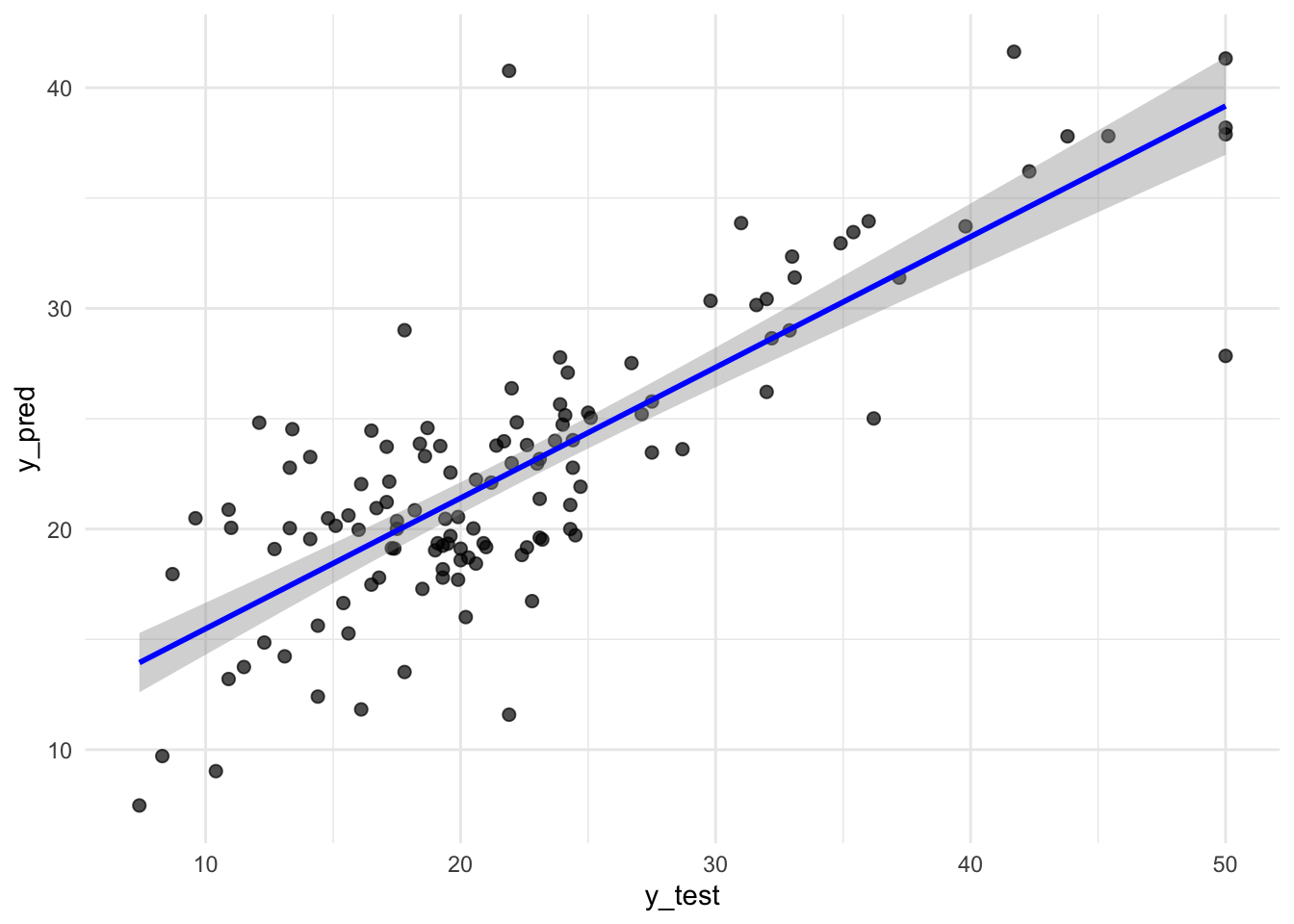
Part 2: Logistic regression
For this part we will use the joined diabetes data since it has a categorical outcome (Diabetes yes or no). We will not use the oral Glucose measurements as predictors since this is literally how you define diabetes, so we’re loading the joined dataset we created in exercise 1, e.g. ‘diabetes_join.xlsx’ or what you have named it. N.B if you did not manage to finish making this dataset or forgot to save it, you can find a copy here: ../out/diabetes_join.Rdata. Navigate to the file in the file window of Rstudio and click on it. Click “Yes” to confirm that the file can be loaded in your environment and check that it has happened.
As the outcome we are studying, Diabetes, is categorical variable we will perform logistic regression. We select serum calcium levels (Serum_ca2), BMI and smoking habits (Smoker) as predictive variables.
- Read in the diabetes_join.xlsx dataset.
diabetes_join <- read_xlsx("../data/exercise1_diabetes_join.xlsx")

head(diabetes_join)
# A tibble: 6 × 11
ID Sex Age BloodPressure BMI PhysicalActivity Smoker Diabetes
<chr> <chr> <dbl> <dbl> <dbl> <dbl> <chr> <dbl>
1 ID_34120 Female 28 75 25.4 92 Never 0
2 ID_27458 Female 55 72 24.6 86 Never 0
3 ID_70630 Male 22 80 24.9 139 Unknown 0
4 ID_13861 Female 56 72 37.1 64 Unknown 1
5 ID_68794 Female 21 62 23 82 Former 0
6 ID_64778 Female 54 76 33.8 63 Smoker 1
# ℹ 3 more variables: Serum_ca2 <dbl>, Married <chr>, Work <chr>- Logistic regression does not allow for any missing values in the outcome variable. Ensure that the variable
Diabetesdoes not have missing values AND that it is a factor variable.
diabetes_df <- diabetes_join %>%
  filter(!is.na(Diabetes)) %>%
mutate(Diabetes= as.factor(Diabetes))- Split your data into training and test data. Take care that the two classes of the outcome variables are represented in both training and test data, and at similar ratios.
set.seed(123)


train <- diabetes_df %>% sample_frac(.75)
test  <- anti_join(diabetes_df, train, by = 'ID')
train_counts <- train[,-1] %>%
dplyr::select(where(is.character)) %>%
pivot_longer(everything(), names_to = "Variable", values_to = "Level") %>%
dplyr::count(Variable, Level, name = "Count")
train_counts# A tibble: 12 × 3
Variable Level Count
<chr> <chr> <int>
1 Married No 126
2 Married Yes 230
3 Sex Female 202
4 Sex Male 154
5 Smoker Former 80
6 Smoker Never 112
7 Smoker Smoker 115
8 Smoker Unknown 49
9 Work Private 189
10 Work Public 106
11 Work Retired 2
12 Work SelfEmployed 59test_counts <- test[,-1] %>%
dplyr::select(where(is.character)) %>%
pivot_longer(everything(), names_to = "Variable", values_to = "Level") %>%
dplyr::count(Variable, Level, name = "Count")
test_counts# A tibble: 12 × 3
Variable Level Count
<chr> <chr> <int>
1 Married No 39
2 Married Yes 79
3 Sex Female 63
4 Sex Male 55
5 Smoker Former 33
6 Smoker Never 31
7 Smoker Smoker 33
8 Smoker Unknown 21
9 Work Private 63
10 Work Public 35
11 Work Retired 2
12 Work SelfEmployed 18- Fit a logistic regression model with
Serum_ca2,BMIandSmokeras predictors andDiabetesas outcome, using your training data.
mod1 <- glm(Diabetes ~ Serum_ca2 + BMI + Smoker, data = train, family = 'binomial')
summary(mod1)
Call:
glm(formula = Diabetes ~ Serum_ca2 + BMI + Smoker, family = "binomial",
    data = train)

Coefficients:
               Estimate Std. Error z value Pr(>|z|)
(Intercept)   -29.66172    9.24103  -3.210  0.00133 **
Serum_ca2       0.62235    0.91791   0.678  0.49777
BMI             0.77975    0.09837   7.927 2.25e-15 ***
SmokerNever    -1.33474    0.63225  -2.111  0.03476 *
SmokerSmoker    1.71880    0.67054   2.563  0.01037 *
SmokerUnknown  -0.27908    0.75901  -0.368  0.71310
---
Signif. codes:  0 '***' 0.001 '**' 0.01 '*' 0.05 '.' 0.1 ' ' 1

(Dispersion parameter for binomial family taken to be 1)

    Null deviance: 493.34  on 355  degrees of freedom
Residual deviance: 122.91  on 350  degrees of freedom
AIC: 134.91

Number of Fisher Scoring iterations: 7- Check the model summary and try to determine whether you could potentially drop one of your variables? If so, make this alternative model and compare it to the original model. Is there a significant loss/gain, i.e. better fit when including the serum calcium levels as predictor?
mod2 <- glm(Diabetes ~ BMI + Smoker, data = train, family = binomial)
summary(mod2)
Call:
glm(formula = Diabetes ~ BMI + Smoker, family = binomial, data = train)

Coefficients:
               Estimate Std. Error z value Pr(>|z|)
(Intercept)   -23.84692    3.07881  -7.745 9.52e-15 ***
BMI             0.78180    0.09873   7.918 2.41e-15 ***
SmokerNever    -1.32566    0.63378  -2.092   0.0365 *
SmokerSmoker    1.64646    0.65738   2.505   0.0123 *
SmokerUnknown  -0.28021    0.75992  -0.369   0.7123
---
Signif. codes:  0 '***' 0.001 '**' 0.01 '*' 0.05 '.' 0.1 ' ' 1

(Dispersion parameter for binomial family taken to be 1)

    Null deviance: 493.34  on 355  degrees of freedom
Residual deviance: 123.38  on 351  degrees of freedom
AIC: 133.38

Number of Fisher Scoring iterations: 7anova(mod1, mod2, test = "Chisq")Analysis of Deviance Table
Model 1: Diabetes ~ Serum_ca2 + BMI + Smoker
Model 2: Diabetes ~ BMI + Smoker
Resid. Df Resid. Dev Df Deviance Pr(>Chi)
1 350 122.91
2 351 123.38 -1 -0.46762 0.4941- Now, use your model to predict Diabetes class based on your test set. What does the output of the prediction mean?
y_pred <- predict(mod2, test, type = "response")- Lets evaluate the performance of our model. As we are performing classification, measures such as mse/rmse will not work, instead we will calculate the accuracy. In order to get the accuracy you must first convert our predictions into Diabetes class labels (e.g. 0 or 1).
y_pred <- as.factor(ifelse(y_pred > 0.5, 1, 0))

caret::confusionMatrix(y_pred, test$Diabetes)
Confusion Matrix and Statistics
Reference
Prediction 0 1
0 60 4
1 2 52
Accuracy : 0.9492
95% CI : (0.8926, 0.9811)
No Information Rate : 0.5254
P-Value [Acc > NIR] : <2e-16
Kappa : 0.8979
Mcnemar's Test P-Value : 0.6831
Sensitivity : 0.9677
Specificity : 0.9286
Pos Pred Value : 0.9375
Neg Pred Value : 0.9630
Prevalence : 0.5254
Detection Rate : 0.5085
Detection Prevalence : 0.5424
Balanced Accuracy : 0.9482
'Positive' Class : 0