Exercise 5 - Solutions

Load packages

library(tidyverse)
library(ModelMetrics)
library(readxl)
library(caTools)
library(car)
library(ggfortify)

Part 1: Linear regression

Load the data boston.csv

df <- as_tibble(read.delim('../data/boston.csv', sep = ','))
head(df)

# A tibble: 6 × 6
     crim indus   nox    rm  medv neighborhood
    <dbl> <dbl> <dbl> <dbl> <dbl> <chr>       
1 0.00632  2.31 0.538  6.58  24   Suburban    
2 0.0273   7.07 0.469  6.42  21.6 Urban       
3 0.0273   7.07 0.469  7.18  34.7 Rural       
4 0.0324   2.18 0.458  7.00  33.4 Urban       
5 0.0690   2.18 0.458  7.15  36.2 Suburban    
6 0.0298   2.18 0.458  6.43  28.7 Suburban

Neighborhood is a categorical variable. We could make it a factor but it will also work as a character column (in the case of using lm).
Split the dataset into test and training data.

# Set seed to ensure reproducibility
set.seed(123)  

#add an ID column to keep track of observations
df$ID <- 1:nrow(df)

train <- df %>% sample_frac(.75)
test  <- anti_join(df, train, by = 'ID')

Fit the model

model <- lm(medv ~ rm + crim + neighborhood, data = train)

summary(model)


Call:
lm(formula = medv ~ rm + crim + neighborhood, data = train)

Residuals:
    Min      1Q  Median      3Q     Max 
-19.920  -3.167  -0.468   2.746  35.052 

Coefficients:
                      Estimate Std. Error t value Pr(>|t|)    
(Intercept)          -25.52560    3.08810  -8.266 2.43e-15 ***
rm                     7.63165    0.49122  15.536  < 2e-16 ***
crim                  -0.22845    0.03525  -6.482 2.86e-10 ***
neighborhoodSuburban   0.07995    0.75050   0.107    0.915    
neighborhoodUrban      3.66323    0.84058   4.358 1.70e-05 ***
---
Signif. codes:  0 '***' 0.001 '**' 0.01 '*' 0.05 '.' 0.1 ' ' 1

Residual standard error: 6.183 on 375 degrees of freedom
Multiple R-squared:  0.5573,    Adjusted R-squared:  0.5525 
F-statistic:   118 on 4 and 375 DF,  p-value: < 2.2e-16

rm and crim have a significant influence on the house price. An increase in the number of rooms increases the price since the coefficient is positive, whereas an increase in crime rate reduces the price. There is a significant difference in price between Rural and Urban zones, but not between Rural and Suburban. Rural is the reference level. Lastly, houses with 0 rooms cost -25k dollar. Perhaps the predictors should be centered before fitting the model around 0 so rm == 0 is the average number of rooms for better interpretability.
Scale the numeric predictor columns and redo the modelling. What has changed?

Hint

There is a scale function, see ?scale().

df <- df %>%
  mutate(across(where(is.numeric), scale, .names = "standardized_{.col}"))

head(df)

# A tibble: 6 × 13
     crim indus   nox    rm  medv neighborhood    ID standardized_crim[,1]
    <dbl> <dbl> <dbl> <dbl> <dbl> <chr>        <int>                 <dbl>
1 0.00632  2.31 0.538  6.58  24   Suburban         1                -0.419
2 0.0273   7.07 0.469  6.42  21.6 Urban            2                -0.417
3 0.0273   7.07 0.469  7.18  34.7 Rural            3                -0.417
4 0.0324   2.18 0.458  7.00  33.4 Urban            4                -0.416
5 0.0690   2.18 0.458  7.15  36.2 Suburban         5                -0.412
6 0.0298   2.18 0.458  6.43  28.7 Suburban         6                -0.417
# ℹ 5 more variables: standardized_indus <dbl[,1]>, standardized_nox <dbl[,1]>,
#   standardized_rm <dbl[,1]>, standardized_medv <dbl[,1]>,
#   standardized_ID <dbl[,1]>

# Set seed to ensure reproducibility
set.seed(123)  

train <- df %>% sample_frac(.75)
test  <- anti_join(df, train, by = 'ID')

model_std <- lm(medv ~ standardized_rm + standardized_crim + neighborhood, data = train)
summary(model_std)


Call:
lm(formula = medv ~ standardized_rm + standardized_crim + neighborhood, 
    data = train)

Residuals:
    Min      1Q  Median      3Q     Max 
-19.920  -3.167  -0.468   2.746  35.052 

Coefficients:
                     Estimate Std. Error t value Pr(>|t|)    
(Intercept)          21.61103    0.52360  41.274  < 2e-16 ***
standardized_rm       5.36213    0.34514  15.536  < 2e-16 ***
standardized_crim    -1.96504    0.30317  -6.482 2.86e-10 ***
neighborhoodSuburban  0.07995    0.75050   0.107    0.915    
neighborhoodUrban     3.66323    0.84058   4.358 1.70e-05 ***
---
Signif. codes:  0 '***' 0.001 '**' 0.01 '*' 0.05 '.' 0.1 ' ' 1

Residual standard error: 6.183 on 375 degrees of freedom
Multiple R-squared:  0.5573,    Adjusted R-squared:  0.5525 
F-statistic:   118 on 4 and 375 DF,  p-value: < 2.2e-16

All significance observations stay the same since scaling can never affect that. The size of the coefficients will usually change since the range of the predictor (that they are multiplied with in the formula) has changed, but their direction stays the same. Now a house with the average number of rooms (rm == 0) costs 21k.

Part 2: Logistic regression

For this part we will use the joined diabetes data since it has a categorical outcome (Diabetes yes or no). We will not use the oral Glucose measurements as predictors since this is literally how you define diabetes, so we’re loading the joined dataset we created in exercise 1, e.g. ‘diabetes_join.xlsx’ or what you have named it.

diabetes_df <- read_excel('../out/diabetes_join.xlsx')
head(diabetes_df)

# A tibble: 6 × 11
  ID    Sex      Age BloodPressure   BMI PhysicalActivity Smoker  Diabetes
  <chr> <chr>  <dbl>         <dbl> <dbl>            <dbl> <chr>   <chr>   
1 9046  Male      34            84  24.7               93 Unknown 0       
2 51676 Male      25            74  22.5              102 Unknown 0       
3 60182 Male      50            80  34.5               98 Unknown 1       
4 1665  Female    27            60  26.3               82 Never   0       
5 56669 Male      35            84  35                 58 Smoker  1       
6 53882 Female    31            78  43.3               59 Smoker  1       
# ℹ 3 more variables: Serum_ca2 <dbl>, Married <chr>, Work <chr>

We choose to make a regression model of Diabetes as predicted by serum calcium levels (Serum_ca2), BMI and smoking habits (Smoker).

We cannot have NA values in our predictors so remove all rows with NAs and save the result into a new dataframe diabetes_nona.

diabetes_nona <- drop_na(diabetes_df)
nrow(diabetes_nona)

[1] 488

nrow(diabetes_df)

[1] 490

Make the outcome variable into a factor if it is not already.

class(diabetes_nona$Diabetes)

[1] "character"

diabetes_nona$Diabetes <- factor(diabetes_nona$Diabetes)
class(diabetes_nona$Diabetes)

[1] "factor"

Scale all numeric predictors. Check your result.

diabetes_nona <- diabetes_nona %>%
  #scale all numeric cols
  mutate(across(where(is.numeric), scale))

head(diabetes_nona)

# A tibble: 6 × 11
  ID    Sex    Age[,1] BloodPressure[,1] BMI[,1] PhysicalActivity[,1] Smoker 
  <chr> <chr>    <dbl>             <dbl>   <dbl>                <dbl> <chr>  
1 9046  Male    0.0166             0.881  -0.820               0.351  Unknown
2 51676 Male   -0.775              0.104  -1.15                0.708  Unknown
3 60182 Male    1.42               0.570   0.646               0.550  Unknown
4 1665  Female -0.599             -0.985  -0.581              -0.0855 Never  
5 56669 Male    0.105              0.881   0.720              -1.04   Smoker 
6 53882 Female -0.247              0.415   1.96               -0.998  Smoker 
# ℹ 4 more variables: Diabetes <fct>, Serum_ca2 <dbl[,1]>, Married <chr>,
#   Work <chr>

Split your data into training and test data. Take care that the two classes of the outcome variable are in the same ratio in both training and test data.

# Set seed to ensure reproducibility
set.seed(123)

split <- sample.split(diabetes_nona$Diabetes, SplitRatio = 0.75)

train <- diabetes_nona[split,]
test <- diabetes_nona[!split,] #! negates the vector, so true becomes false and vice verse

count(train,Diabetes)

# A tibble: 2 × 2
  Diabetes     n
  <fct>    <int>
1 0          182
2 1          184

count(test, Diabetes)

# A tibble: 2 × 2
  Diabetes     n
  <fct>    <int>
1 0           61
2 1           61

Fit a regression model with Serum_ca2, BMI and Smoker as predictors. Check the model summary.

mod1 <- glm(Diabetes ~ Serum_ca2 + BMI + Smoker, data = train, family = binomial)
summary(mod1)


Call:
glm(formula = Diabetes ~ Serum_ca2 + BMI + Smoker, family = binomial, 
    data = train)

Deviance Residuals: 
    Min       1Q   Median       3Q      Max  
-2.9170  -0.1187   0.0004   0.2087   1.9340  

Coefficients:
              Estimate Std. Error z value Pr(>|z|)    
(Intercept)    -0.1099     0.4541  -0.242   0.8088    
Serum_ca2      -0.1028     0.2100  -0.490   0.6244    
BMI             5.2882     0.6628   7.979 1.48e-15 ***
SmokerNever    -1.3338     0.6335  -2.105   0.0353 *  
SmokerSmoker    1.2924     0.6277   2.059   0.0395 *  
SmokerUnknown  -0.1880     0.6831  -0.275   0.7832    
---
Signif. codes:  0 '***' 0.001 '**' 0.01 '*' 0.05 '.' 0.1 ' ' 1

(Dispersion parameter for binomial family taken to be 1)

    Null deviance: 507.37  on 365  degrees of freedom
Residual deviance: 132.68  on 360  degrees of freedom
AIC: 144.68

Number of Fisher Scoring iterations: 7

Create a second model with only BMI and Smoker as predictors. Compare the fit of your second model to the first one (including Serum_ca2). Is there a significant gain, i.e. better fit when including the serum calcium levels as predictor? Which model do you think is better?

mod2 <- glm(Diabetes ~ BMI + Smoker, data = train, family = binomial)
summary(mod2)


Call:
glm(formula = Diabetes ~ BMI + Smoker, family = binomial, data = train)

Deviance Residuals: 
    Min       1Q   Median       3Q      Max  
-2.9122  -0.1224   0.0004   0.1977   1.8537  

Coefficients:
              Estimate Std. Error z value Pr(>|z|)    
(Intercept)    -0.1177     0.4532  -0.260   0.7951    
BMI             5.2616     0.6557   8.025 1.02e-15 ***
SmokerNever    -1.3237     0.6309  -2.098   0.0359 *  
SmokerSmoker    1.3356     0.6233   2.143   0.0321 *  
SmokerUnknown  -0.1545     0.6781  -0.228   0.8197    
---
Signif. codes:  0 '***' 0.001 '**' 0.01 '*' 0.05 '.' 0.1 ' ' 1

(Dispersion parameter for binomial family taken to be 1)

    Null deviance: 507.37  on 365  degrees of freedom
Residual deviance: 132.92  on 361  degrees of freedom
AIC: 142.92

Number of Fisher Scoring iterations: 7

anova(mod1, mod2, test = "Chisq")

Analysis of Deviance Table

Model 1: Diabetes ~ Serum_ca2 + BMI + Smoker
Model 2: Diabetes ~ BMI + Smoker
  Resid. Df Resid. Dev Df Deviance Pr(>Chi)
1       360     132.68                     
2       361     132.92 -1 -0.23882   0.6251

The likelihood ratio test between the two models has an insignificant p-value. This means there is no evidence that including Serum_ca2 improves the fit of the model. The second model mod2 is therefore preferable.

Part 3: Clustering

In this part we will run clustering on the joined diabetes dataset from exercise 1. Load it here if you don’t have it already from Part 2.

#in case
diabetes_df <- read_excel('../out/diabetes_join.xlsx')
head(diabetes_df)

# A tibble: 6 × 11
  ID    Sex      Age BloodPressure   BMI PhysicalActivity Smoker  Diabetes
  <chr> <chr>  <dbl>         <dbl> <dbl>            <dbl> <chr>   <chr>   
1 9046  Male      34            84  24.7               93 Unknown 0       
2 51676 Male      25            74  22.5              102 Unknown 0       
3 60182 Male      50            80  34.5               98 Unknown 1       
4 1665  Female    27            60  26.3               82 Never   0       
5 56669 Male      35            84  35                 58 Smoker  1       
6 53882 Female    31            78  43.3               59 Smoker  1       
# ℹ 3 more variables: Serum_ca2 <dbl>, Married <chr>, Work <chr>

Run the k-means clustering algorithm with 4 centers on the data. Consider which columns you can use and if you have to manipulate them before. If you get an error, check whether you have values that might not be admissible, such as NA.

# Set seed to ensure reproducibility
set.seed(123)  

#run kmeans
kmeans_res <- diabetes_df %>%
  select(where(is.numeric)) %>%
  #drop missing values
  drop_na() %>%
  #scale all numeric cols
  mutate(across(where(is.numeric), scale)) %>%
  kmeans(centers = 4, nstart = 25)

kmeans_res

K-means clustering with 4 clusters of sizes 121, 105, 121, 141

Cluster means:
         Age BloodPressure        BMI PhysicalActivity    Serum_ca2
1 -0.5286070    -0.3058681 -0.6167955        0.3163233  1.009157782
2 -0.5664483    -0.3764116 -0.8001807        0.9728678 -0.787111758
3  1.3679241     0.8087592  0.3267171       -0.3222905 -0.009092463
4 -0.2984418    -0.1512525  0.8448118       -0.7193553 -0.272065028

Clustering vector:
  [1] 1 1 3 2 4 4 3 3 3 3 2 1 1 1 1 4 1 3 2 3 2 3 1 4 4 4 2 4 1 2 1 2 1 3 1 1 3
 [38] 1 4 2 4 4 1 1 4 1 4 4 2 4 1 4 1 2 2 3 4 2 3 1 4 3 4 2 4 1 2 1 1 1 1 2 2 3
 [75] 2 1 2 4 4 1 1 4 1 1 2 1 1 3 4 2 2 3 2 2 4 4 3 1 4 4 1 4 1 2 1 4 3 3 1 4 3
[112] 4 3 2 2 2 2 2 1 3 3 2 2 4 3 2 4 1 3 3 1 2 1 3 4 1 2 3 2 1 3 3 2 1 2 3 1 2
[149] 4 3 1 2 4 4 3 4 4 4 4 1 3 4 4 4 1 1 3 2 1 2 1 1 4 1 4 2 2 1 3 2 4 4 3 2 2
[186] 3 1 4 3 1 1 2 1 3 2 3 3 4 1 2 3 2 3 4 4 3 1 3 3 4 4 4 3 2 2 1 1 4 3 3 4 3
[223] 2 4 2 3 4 2 3 4 3 1 4 3 3 2 4 3 2 1 3 3 3 2 2 4 1 1 2 4 3 3 4 4 2 4 4 1 4
[260] 1 2 1 4 4 4 1 2 3 3 1 4 1 3 1 1 4 2 4 3 3 4 3 3 4 1 3 4 3 4 3 1 4 4 3 2 3
[297] 3 2 3 4 4 2 1 4 4 2 3 1 4 1 2 2 1 2 2 3 4 1 4 3 1 4 4 3 4 4 3 4 1 4 2 2 2
[334] 1 3 2 1 3 1 3 4 4 4 1 1 1 2 4 4 4 2 2 4 4 4 1 3 4 3 4 1 3 1 3 1 1 4 2 2 3
[371] 4 1 2 4 4 2 4 2 4 3 3 4 3 1 2 3 4 4 1 2 4 1 2 2 3 1 1 2 2 2 3 4 3 1 3 4 4
[408] 3 2 3 4 4 1 1 4 4 3 3 4 3 2 4 4 4 1 4 2 1 3 4 1 4 2 3 4 1 1 4 1 1 2 3 2 3
[445] 4 1 3 3 3 2 2 3 3 2 4 4 1 3 3 3 4 1 3 1 3 1 1 3 1 2 1 4 1 1 3 4 4 2 2 4 2
[482] 2 3 3 4 1 4 3

Within cluster sum of squares by cluster:
[1] 317.4167 315.8628 396.1259 367.9939
 (between_SS / total_SS =  42.6 %)

Available components:

[1] "cluster"      "centers"      "totss"        "withinss"     "tot.withinss"
[6] "betweenss"    "size"         "iter"         "ifault"

Check whether the data you have run k-means on has the same number of rows as the dataframe with meta information, e.g. whether the person had diabetes. If they are not aligned, create a dataframe with Diabetes info that matches the dataframe you ran clustering on.

Hint

drop_na() takes an argument that tells which columns to look at for NA values.

The full data:

nrow(diabetes_df)

[1] 490

How many rows did we run clustering on?

diabetes_df %>%
  select(where(is.numeric)) %>%
  #drop missing values
  drop_na() %>%
  #scale all numeric cols
  mutate(across(where(is.numeric), scale)) %>%
  nrow()

[1] 488

We could also have checked the length of kmeans_res$cluster:

length(kmeans_res$cluster)

[1] 488

So we have omitted some rows. We need to omit the same rows from the original dataframe so our k-means clustering results are aligned with it.

diabetes_df <- diabetes_df %>%
  drop_na(where(is.numeric))
nrow(diabetes_df)

[1] 488

Visualize the results of your clustering.

We first need to calculate a PCA. This is basically the same we have done in exercise 3B.

pca_res <- diabetes_df %>%
  select(where(is.numeric)) %>%
  #drop missing values
  drop_na() %>%
  #scale all numeric cols
  mutate(across(where(is.numeric), scale)) %>%
  prcomp()

Now we project the k-means centroids in the PCA space

#project cluster centers from kmeans into the pca space
centers_pca <- predict(pca_res, newdata = kmeans_res$centers) %>% as.data.frame()
# Label clusters
centers_pca$cluster <- as.factor(1:nrow(centers_pca))  
centers_pca

         PC1         PC2        PC3         PC4         PC5 cluster
1  0.9517476 -0.08349116 -0.9526042 -0.09077825  0.20829660       1
2  1.3335463  0.41329140  0.8435674 -0.05601768 -0.07039558       2
3 -1.3718134  0.80239970 -0.1598088  0.41230331 -0.12147179       3
4 -0.6325844 -0.92470588  0.3264354 -0.23420338 -0.02208699       4

And add cluster assignments to the diabetes_df:

diabetes_df$Cluster <- factor(kmeans_res$cluster)

Finally we can plot:

autoplot(pca_res, data = diabetes_df, color = 'Cluster',
         loadings = TRUE, loadings.colour = "grey30", 
         loadings.label.colour = "black",
         loadings.label = TRUE, loadings.label.size = 3.5,
         scale = 0) + 
  theme_minimal() +
  labs(title = "PCA of Diabetes Dataset") +
  # Cluster centers
  geom_point(data = centers_pca, aes(x = PC1, y = PC2, color = cluster),
             shape = 8, size = 6, stroke = 2)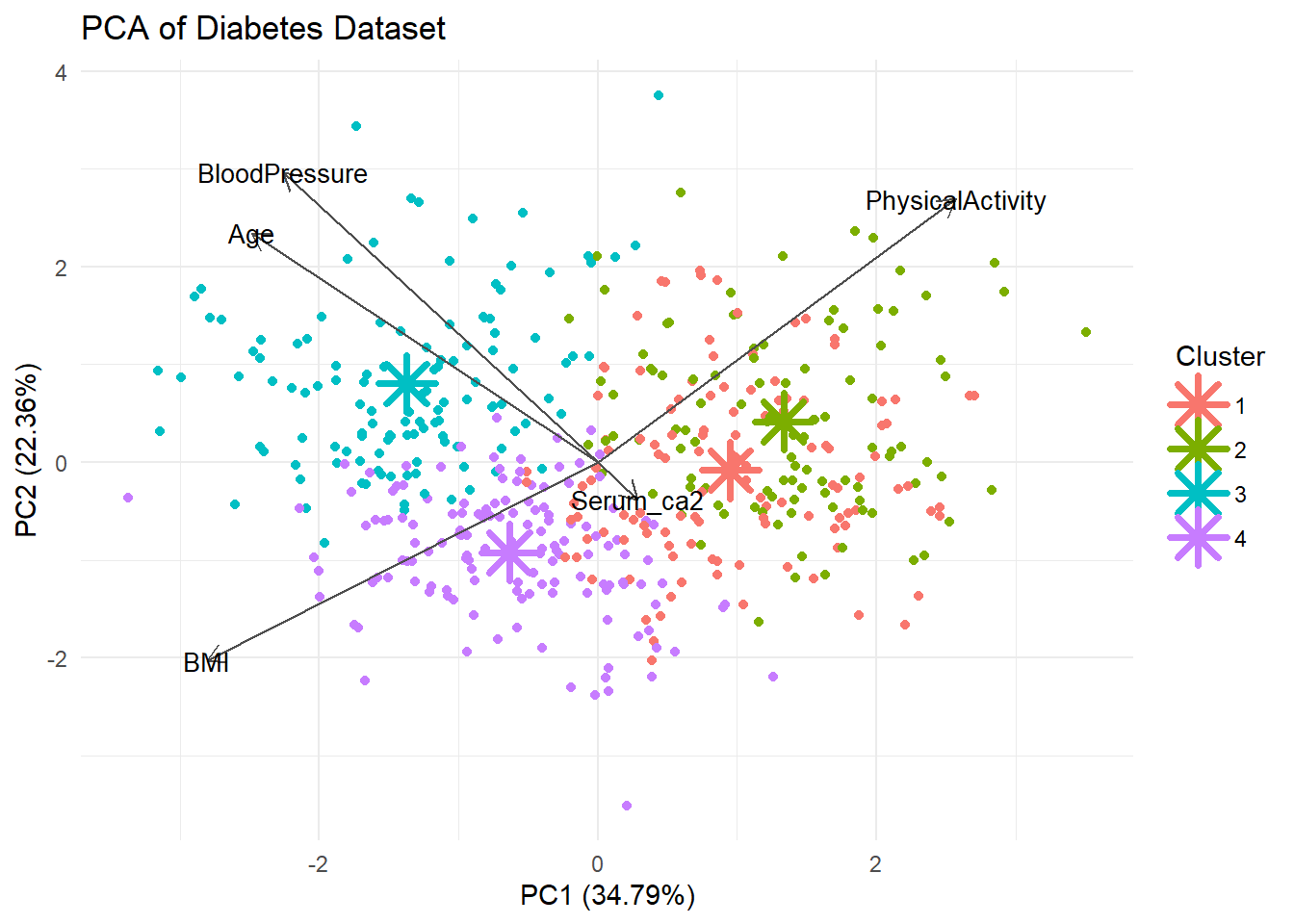

Well the separation was not that good in exercise 3B so perhaps we should not expect very clean clusters.

Investigate the best number of clusters.

library(factoextra)

Warning: pakke 'factoextra' blev bygget under R version 4.2.3

Welcome! Want to learn more? See two factoextra-related books at https://goo.gl/ve3WBa

diabetes_df %>%
  select(where(is.numeric)) %>%
  #drop missing values
  drop_na() %>%
  #scale all numeric cols
  mutate(across(where(is.numeric), scale)) %>%
  fviz_nbclust(kmeans, method = "wss")

diabetes_df %>%
  select(where(is.numeric)) %>%
  #drop missing values
  drop_na() %>%
  #scale all numeric cols
  mutate(across(where(is.numeric), scale)) %>%
  fviz_nbclust(kmeans, method = "silhouette")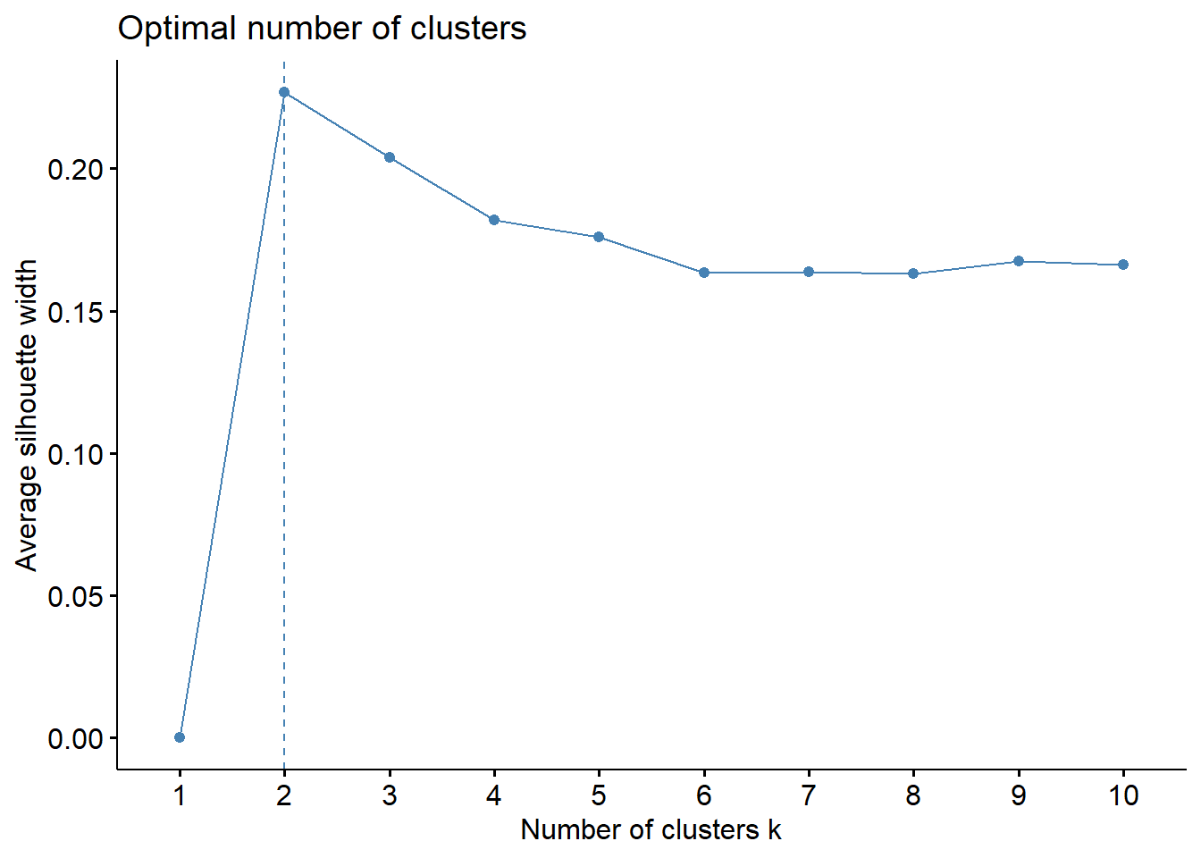

diabetes_df %>%
  select(where(is.numeric)) %>%
  #drop missing values
  drop_na() %>%
  #scale all numeric cols
  mutate(across(where(is.numeric), scale)) %>%
  fviz_nbclust(kmeans, method = "gap_stat")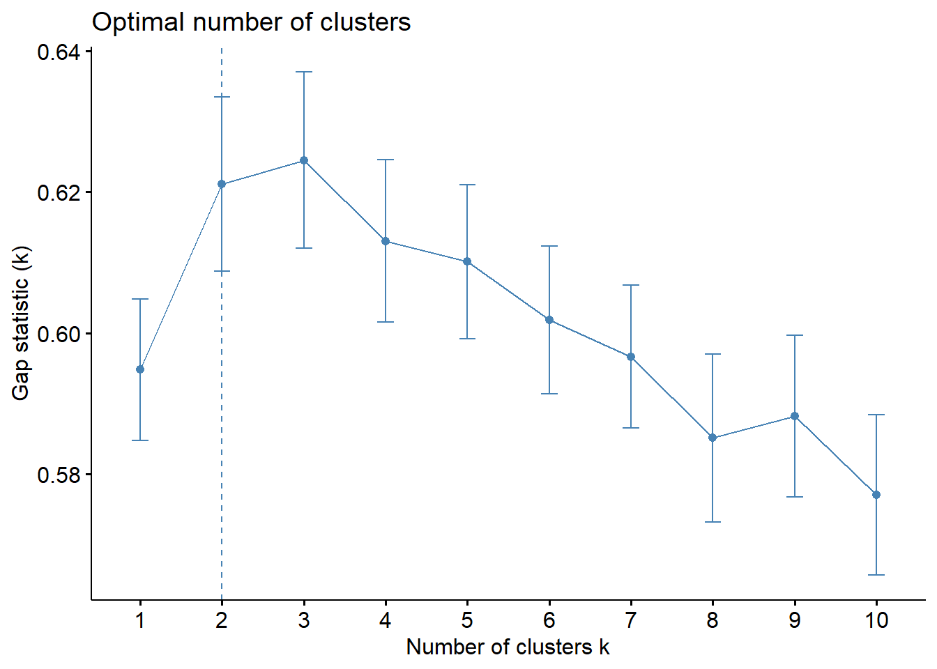

The elbow is not very clear but the silhouette and gap statistic favor 2 clusters - which kind of makes sense since we have two outcomes, diabetic and non-diabetic.

Re-do the clustering (plus visualization) with that number.

# Set seed to ensure reproducibility
set.seed(123)  

#run kmeans
kmeans_res <- diabetes_df %>%
  select(where(is.numeric)) %>%
  #drop missing values
  drop_na() %>%
  #scale all numeric cols
  mutate(across(where(is.numeric), scale)) %>%
  kmeans(centers = 2, nstart = 25)

kmeans_res

K-means clustering with 2 clusters of sizes 257, 231

Cluster means:
         Age BloodPressure        BMI PhysicalActivity  Serum_ca2
1  0.4697155     0.3538870  0.6621866       -0.5424263 -0.1002325
2 -0.5225839    -0.3937184 -0.7367184        0.6034786  0.1115140

Clustering vector:
  [1] 2 2 1 2 1 1 1 1 1 1 2 2 2 2 2 1 2 1 2 1 2 1 1 1 1 1 2 1 2 2 2 2 2 1 2 2 1
 [38] 1 2 2 1 1 1 1 1 2 2 1 2 1 2 1 2 2 2 1 1 2 1 2 1 1 1 2 1 2 2 2 2 2 2 2 2 1
 [75] 2 2 2 1 1 2 2 2 2 2 2 1 2 1 1 2 2 1 2 2 1 1 1 2 1 1 2 1 2 2 2 1 1 1 2 1 1
[112] 2 1 2 2 2 2 2 2 2 1 2 2 1 1 2 1 2 1 1 2 2 2 1 1 2 2 1 2 2 1 1 2 2 2 1 2 1
[149] 1 1 2 2 2 1 1 1 1 1 1 2 1 2 2 1 1 2 1 2 2 2 1 2 1 2 1 2 2 2 1 2 1 1 1 2 2
[186] 2 2 1 1 2 1 2 2 1 2 1 1 1 2 2 1 2 1 1 1 1 2 1 1 1 1 1 1 2 2 2 2 1 1 1 1 1
[223] 2 1 2 1 1 2 1 1 1 2 1 1 1 2 2 1 2 2 1 1 1 1 2 1 2 2 2 1 1 1 2 1 2 1 1 2 1
[260] 2 2 2 1 1 1 2 2 1 1 2 1 2 1 2 2 1 2 1 1 1 1 1 1 1 2 1 1 1 1 1 2 1 1 1 2 1
[297] 1 2 1 1 1 2 2 1 1 2 1 2 1 2 2 1 2 2 2 1 1 2 1 1 2 1 1 1 1 2 1 1 2 1 2 2 2
[334] 2 1 2 2 1 2 1 1 1 1 2 2 2 2 1 1 1 2 2 1 1 1 2 1 1 1 1 2 1 2 1 2 2 1 2 2 1
[371] 1 2 2 1 1 2 1 1 1 1 1 1 1 2 1 1 1 1 2 2 2 2 2 2 1 2 2 2 2 2 1 1 1 2 1 1 2
[408] 1 2 1 1 1 2 2 2 1 1 1 1 2 2 2 1 1 2 1 2 2 1 1 2 1 2 2 1 1 1 2 2 2 2 1 2 1
[445] 1 2 1 1 1 2 2 1 1 2 1 1 1 2 2 1 1 2 1 2 1 2 2 1 2 2 2 1 2 2 1 1 1 2 2 1 2
[482] 2 1 1 1 2 1 1

Within cluster sum of squares by cluster:
[1] 959.9630 883.9897
 (between_SS / total_SS =  24.3 %)

Available components:

[1] "cluster"      "centers"      "totss"        "withinss"     "tot.withinss"
[6] "betweenss"    "size"         "iter"         "ifault"

#project cluster centers from kmeans into the pca space
centers_pca <- predict(pca_res, newdata = kmeans_res$centers) %>% as.data.frame()
# Label clusters
centers_pca$cluster <- as.factor(1:nrow(centers_pca))  
centers_pca

        PC1        PC2         PC3          PC4         PC5 cluster
1 -1.032372 -0.1214937  0.05219972  0.003763692 -0.07308096       1
2  1.148570  0.1351683 -0.05807502 -0.004187311  0.08130652       2

diabetes_df$Cluster <- factor(kmeans_res$cluster)

autoplot(pca_res, data = diabetes_df, color = 'Cluster',
         loadings = TRUE, loadings.colour = "grey30", 
         loadings.label.colour = "black",
         loadings.label = TRUE, loadings.label.size = 3.5,
         scale = 0) + 
  theme_minimal() +
  labs(title = "PCA of Diabetes Dataset") +
  # Cluster centers
  geom_point(data = centers_pca, aes(x = PC1, y = PC2, color = cluster),
             shape = 8, size = 6, stroke = 2)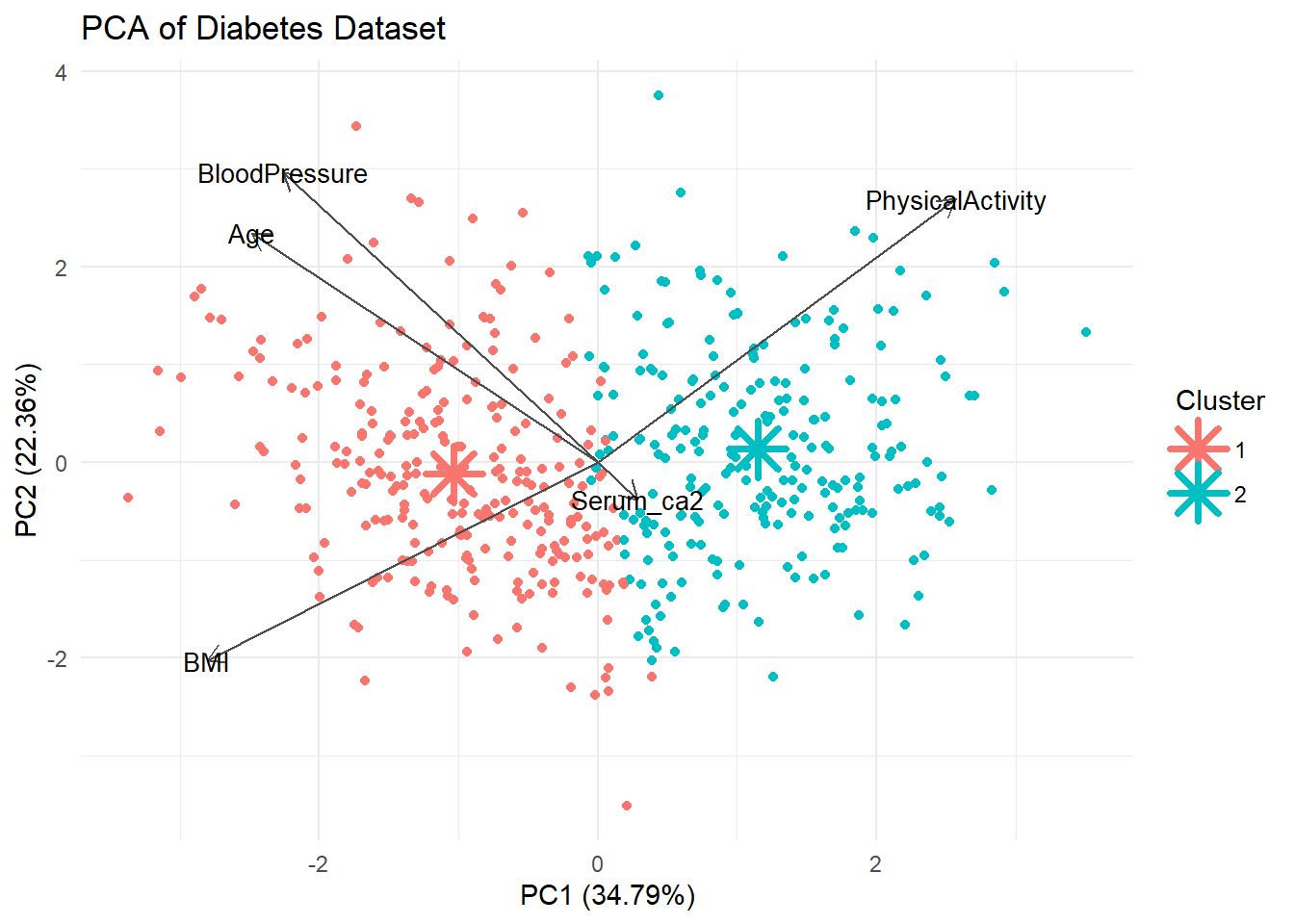

Extra exercises

e1. Find the best single predictor in the Diabetes dataset. This is done by comparing the null model (no predictors) to all possible models with one predictor, i.e. outcome ~ predictor, outcome ~ predictor2, ect. The null model can be formulated like so: outcome ~ 1 (only the intercept). Fit all possible one predictor models and compare their fit to the null model with a likelihood ratio test. Find the predictor with the lowest p-value in the likelihood ratio test. This can be done in a loop in order to avoid writing out all models.

Hint

To use a formula with a variable you will need to combine the literal part and the variable with paste, e.g. paste("Outcome ~", my_pred).

# Define the null model (intercept-only model)
null_model <- glm(Diabetes ~ 1, data = train, family = binomial)

# Get predictor names (excluding the outcome variable)
predictors <- setdiff(names(diabetes_nona), c("Diabetes", "ID"))

# Initialize an empty data frame to store results
results <- data.frame(Predictor = character(), ChiSq = numeric(), P_Value = numeric(), stringsAsFactors = FALSE)

# Loop through each predictor and fit a logistic regression model
for (pred in predictors) {
  
  # Fit model with single predictor
  model_pred <- glm(paste("Diabetes ~", pred), data = train, family = binomial)
  
  # Perform Likelihood Ratio Test
  test_result <- anova(null_model, model_pred, test = "Chisq")
  
  # Extract Chi-square statistic and p-value
  chi_sq <- test_result$Deviance[2]  # The second row corresponds to the predictor model
  p_value <- test_result$`Pr(>Chi)`[2]
  
  # Store results
  results <- rbind(results, data.frame(Predictor = pred, ChiSq = chi_sq, P_Value = p_value))
}

# Print the results sorted by p-value
results <- results %>% arrange(P_Value)
print(results)

         Predictor       ChiSq      P_Value
1              BMI 353.0033684 9.399861e-79
2 PhysicalActivity 174.3147338 8.449925e-40
3           Smoker  69.2823192 6.080298e-15
4              Age  30.2674741 3.763850e-08
5    BloodPressure  13.6648488 2.185065e-04
6             Work   6.6505603 8.391019e-02
7          Married   2.6869823 1.011713e-01
8              Sex   1.8470863 1.741227e-01
9        Serum_ca2   0.7986775 3.714891e-01

e2. Write a function that handles visualization of k-means clustering results. Think about which information you need to pass and what it should return.