library(tidyverse)Exercise 3 B - Solutions
Getting started
- Load packages.
- Load data from the
.rdsfile you created in Exercise 2.
diabetes_glucose <- read_rds('../out/diabetes_glucose.rds')
head(diabetes_glucose)
# A tibble: 6 × 12
ID Sex Age BloodPressure BMI PhysicalActivity Smoker Diabetes
<fct> <chr> <dbl> <dbl> <dbl> <dbl> <chr> <chr>
1 9046 Male 34 84 24.7 93 Unknown 0
2 51676 Male 25 74 22.5 102 Unknown 0
3 60182 Male 50 80 34.5 98 Unknown 1
4 1665 Female 27 60 26.3 82 Never 0
5 56669 Male 35 84 35 58 Smoker 1
6 53882 Female 31 78 43.3 59 Smoker 1
# ℹ 4 more variables: Serum_ca2 <dbl>, Married <chr>, Work <chr>, OGTT <list>Plotting - Part 3: PCA
For this exercise we will use this tutorial to make a principal component analysis (PCA). First, we perform some preprocessing to get our data into the right format.
- Let’s start by unnesting the OGTT data and using pivot wider so that each Glucose measurement time point gets its own column (again).
diabetes_glucose_unnest <-  diabetes_glucose %>%
  unnest(OGTT) %>%
  pivot_wider(names_from = Measurement,
              values_from = `Glucose (mmol/L)`,
              names_prefix = "Glucose_")

diabetes_glucose_unnest
# A tibble: 490 × 14
ID Sex Age BloodPressure BMI PhysicalActivity Smoker Diabetes
<fct> <chr> <dbl> <dbl> <dbl> <dbl> <chr> <chr>
1 9046 Male 34 84 24.7 93 Unknown 0
2 51676 Male 25 74 22.5 102 Unknown 0
3 60182 Male 50 80 34.5 98 Unknown 1
4 1665 Female 27 60 26.3 82 Never 0
5 56669 Male 35 84 35 58 Smoker 1
6 53882 Female 31 78 43.3 59 Smoker 1
7 10434 Male 52 86 33.3 58 Never 1
8 27419 Female 54 78 35.2 74 Former 1
9 60491 Female 41 90 39.8 67 Smoker 1
10 12109 Female 36 82 30.8 81 Smoker 1
# ℹ 480 more rows
# ℹ 6 more variables: Serum_ca2 <dbl>, Married <chr>, Work <chr>,
# Glucose_0 <dbl>, Glucose_60 <dbl>, Glucose_120 <dbl>- Have a look at your unnested diabetes data set. Can you use all the variables to perform PCA? Subset the dataset to only include the relevant variables.
Hint
PCA can only be performed on numerical values. Extract these (except ID!) from the dataset. Numerical columns can easily be selected with the where(is.numeric) helper.
Extract the numerical columns, including the OGTT measurements.
diabetes_glucose_numerical <- diabetes_glucose_unnest %>%
  select(where(is.numeric))

diabetes_glucose_numerical
# A tibble: 490 × 8
Age BloodPressure BMI PhysicalActivity Serum_ca2 Glucose_0 Glucose_60
<dbl> <dbl> <dbl> <dbl> <dbl> <dbl> <dbl>
1 34 84 24.7 93 9.8 6.65 8.04
2 25 74 22.5 102 9.5 4.49 5.40
3 50 80 34.5 98 9.4 12.9 14.3
4 27 60 26.3 82 9 5.76 6.52
5 35 84 35 58 9.3 10.8 16.2
6 31 78 43.3 59 9.6 11.1 12.8
7 52 86 33.3 58 9.1 10.4 14.7
8 54 78 35.2 74 9.3 6.79 10.1
9 41 90 39.8 67 9.1 7.39 10.3
10 36 82 30.8 81 9.5 11.6 13.0
# ℹ 480 more rows
# ℹ 1 more variable: Glucose_120 <dbl>- PCA cannot handle NA’s in the dataset. Remove all rows with NA in any column in your numerical subset. Then, go back to the original unnested data
diabetes_glucose_unnest(or what you have called it) and also here drop rows that have NAs in the numerical columns (so the same rows you dropped from the numeric subset).This is important because we want to use (categorical) columns present in the original data to later color the resulting PCA, so the two dataframes (original and only numeric columns) need to be aligned and contain the same rows.
diabetes_glucose_numerical <- drop_na(diabetes_glucose_numerical)
nrow(diabetes_glucose_numerical)
[1] 488Align original data.
diabetes_glucose_unnest <- diabetes_glucose_unnest %>%
  drop_na(colnames(diabetes_glucose_numerical))
nrow(diabetes_glucose_unnest)
[1] 488Now our data is ready to make a PCA.
- Calculate the PCA by running
prcompon our prepared data (see the tutorial). Then, create a plot of the resulting PCA (also shown in tutorial).
library(ggfortify)

pca_res <- prcomp(diabetes_glucose_numerical, scale. = TRUE)

autoplot(pca_res)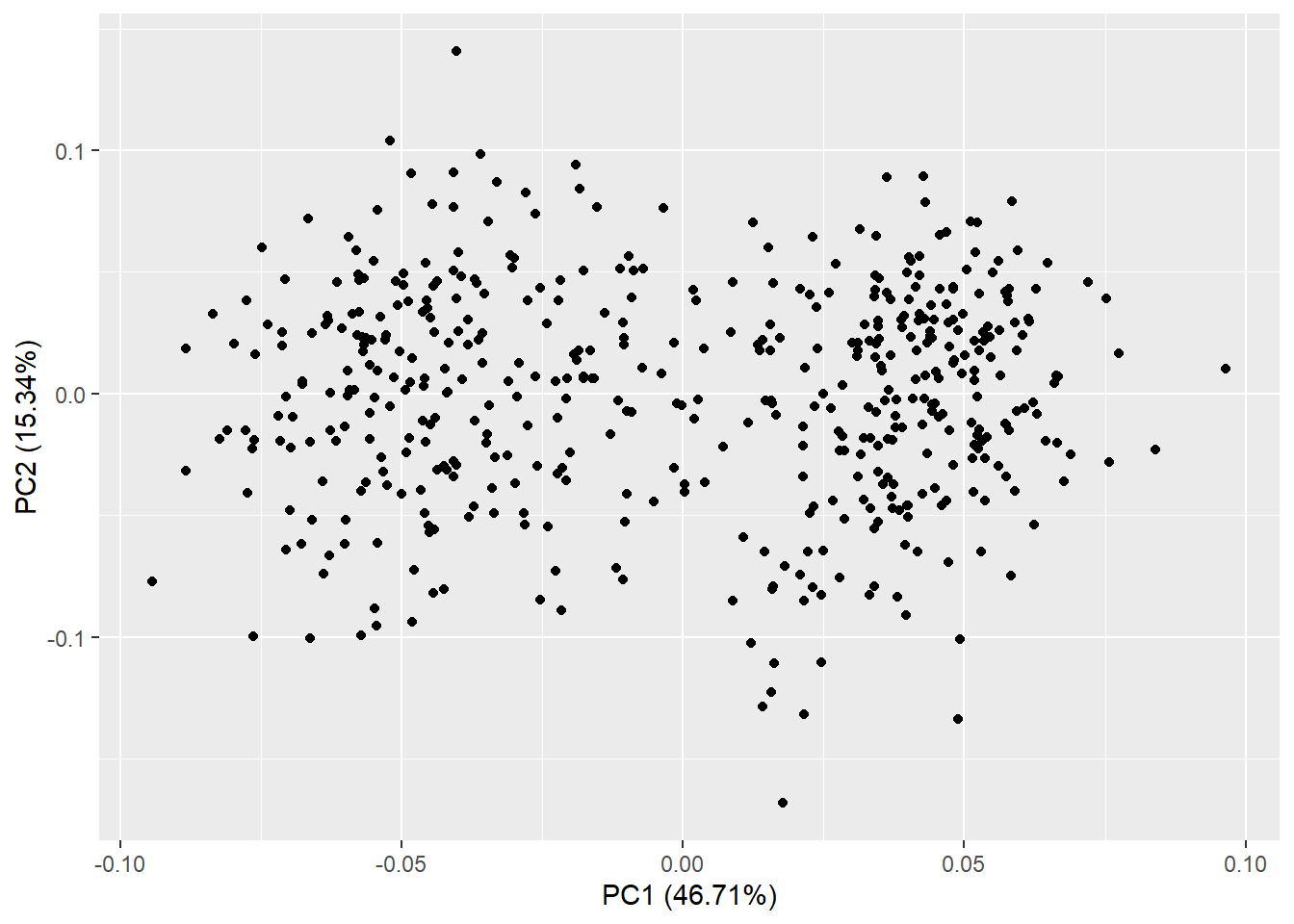
- Color your PCA plot and add loadings. Think about which variable you want to color by. Remember to refer to the dataset that has this variable (probably not your numeric subset!)
autoplot(pca_res, data = diabetes_glucose_unnest, colour = 'Diabetes',
         loadings = TRUE, loadings.colour = 'black',
         loadings.label = TRUE, loadings.label.size = 3)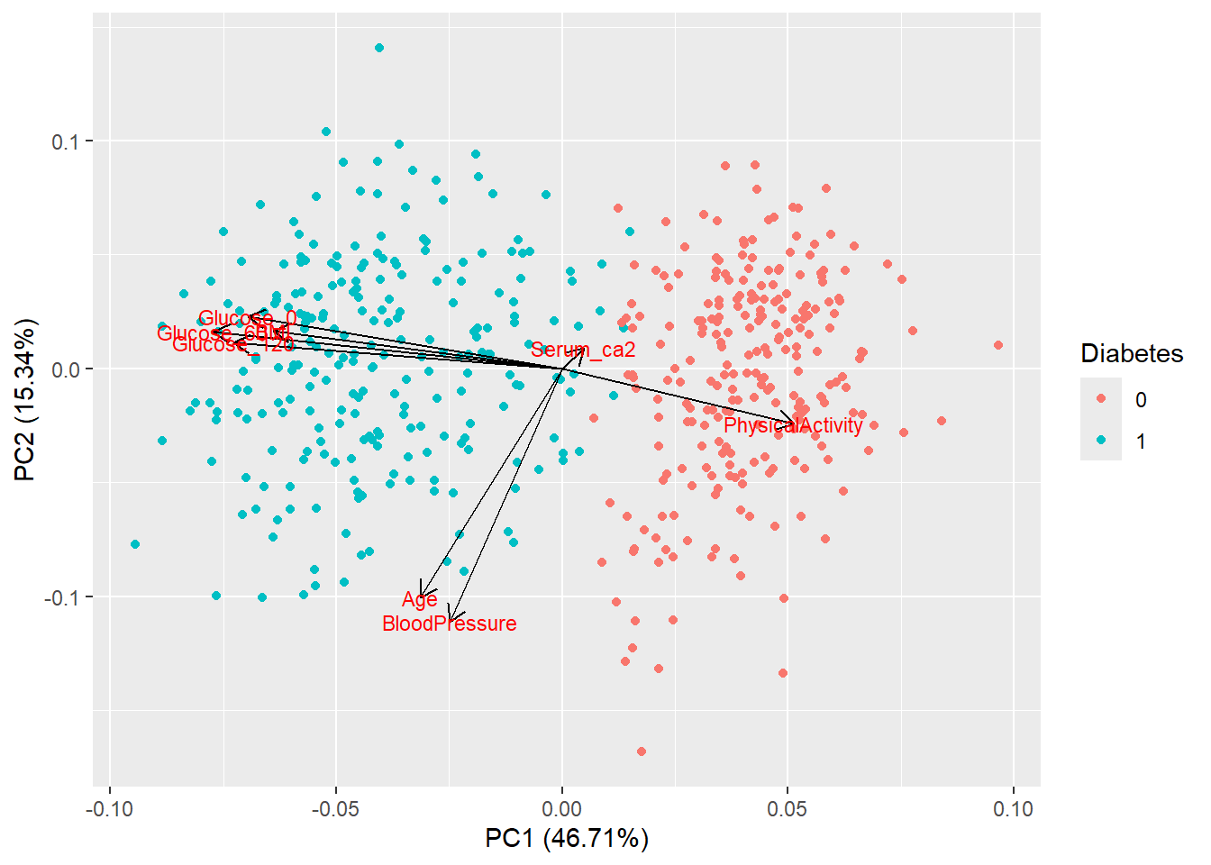
- Add a ggplot
themeand title to your plot and save it.
autoplot(pca_res, data = diabetes_glucose_unnest, colour = "Diabetes",
         loadings = TRUE, loadings.colour = "grey30", loadings.label.colour = "black",
         loadings.label = TRUE, loadings.label.size = 3.5) +
  theme_minimal() +
  labs(title = "PCA of Diabetes Dataset")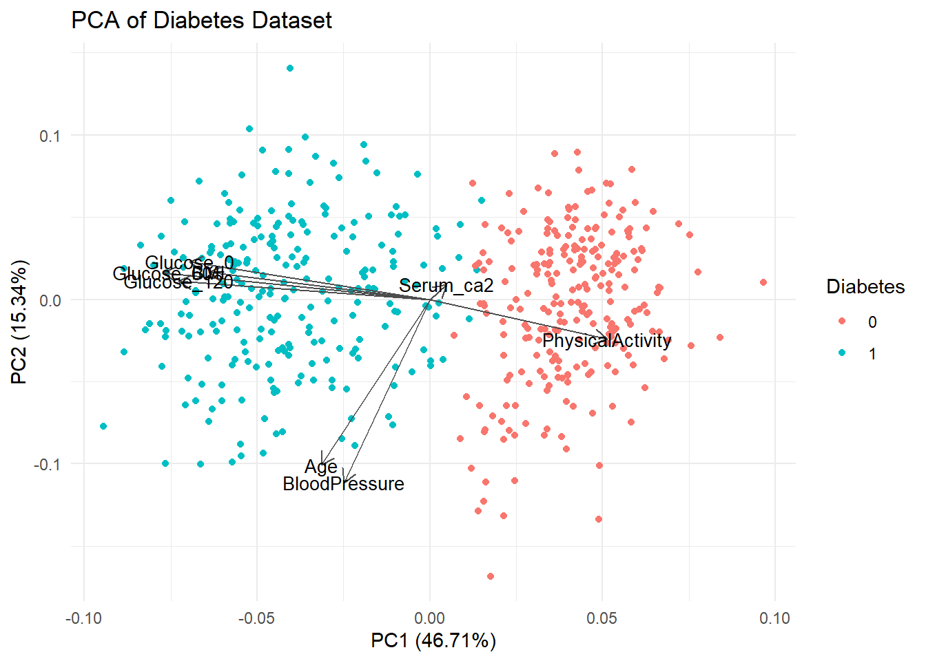
ggsave('../figures/PCA_diabetes.png', width = 7, height = 5)- Calculate the variance explained by each of the PC’s using the following formula:
\[ \text{Variance Explained} = \frac{\text{sdev}^2}{\sum \text{sdev}^2} \times 100 \]
Hint
You can access the standard deviation from the PCA object like this: pca_res$sdev.
variance_explained <- ((pca_res$sdev^2) / sum(pca_res$sdev^2)) * 100
variance_explained
[1] 46.70757453 15.34011234 12.49983700 8.74106790 7.52024687 5.14424345
[7] 3.95709895 0.08981894- Create a two column data-frame with the names of the PC’s (PC1, PC2, ect) in one column and the variance explained by that PC in the other column.
df_variance_explained <- tibble(PC = c(paste0('PC', 1:length(variance_explained))),
                                variance_explained = variance_explained)

df_variance_explained
# A tibble: 8 × 2
PC variance_explained
<chr> <dbl>
1 PC1 46.7
2 PC2 15.3
3 PC3 12.5
4 PC4 8.74
5 PC5 7.52
6 PC6 5.14
7 PC7 3.96
8 PC8 0.0898- Now create a bar plot (using
geom_col), showing for each PC the amount of explained variance. This type of plot is called a scree plot.
df_variance_explained %>%
  ggplot(aes(x = PC,
             y = variance_explained))+
  geom_col() +
  labs(title = "Varinace explained for each PC",
       y = "Variance Explained")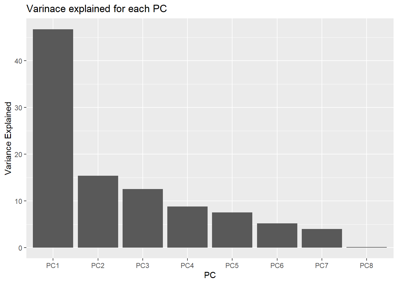
- Lastly, render you quarto document and review the resulting html file.
Extra exercises
e1. The Oral Glucose Tolerance Test is used to diagnose diabetes so we are not surprised that it separates the dataset well. In this part, we will look at a PCA without the OGTT measurements and see how we fare. Omit the Glucose measurement columns, calculate a PCA and create the plot.
pca_no_gluc <-diabetes_glucose_numerical %>%
  select(-Glucose_0,-Glucose_60,-Glucose_120) %>%
prcomp(scale. = TRUE)autoplot(pca_no_gluc, data = diabetes_glucose_unnest, colour = "Diabetes",
loadings = TRUE, loadings.colour = "grey30", loadings.label.colour = "black",
loadings.label = TRUE, loadings.label.size = 3.5) +
theme_minimal() +
labs(title = "PCA of Diabetes Dataset")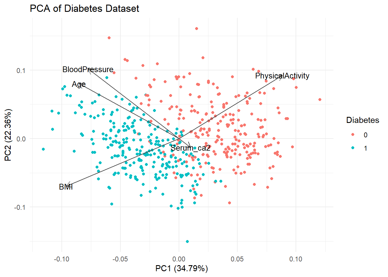
Without the Glucose measurement data our strongest separating variables are BMI and Physical Activity.