library(tidyverse)
library(readxl)Exercise 1 - Solutions: Data Cleanup (Base R and Tidyverse)
Getting started
- Load packages.
- Load in the
diabetes_clinical_toy_messy.xlsxdata set.
diabetes_clinical <- read_excel('../data/diabetes_clinical_toy_messy.xlsx')
head(diabetes_clinical)
# A tibble: 6 × 9
ID Sex Age BloodPressure BMI PhysicalActivity Smoker Diabetes
<dbl> <chr> <dbl> <dbl> <dbl> <dbl> <chr> <dbl>
1 9046 Male 34 84 24.7 93 Unknown 0
2 51676 Male 25 74 22.5 102 Unknown 0
3 31112 Male 30 0 32.3 75 Former 1
4 60182 Male 50 80 34.5 98 Unknown 1
5 1665 Female 27 60 26.3 82 Never 0
6 56669 Male 35 84 35 58 Smoker 1
# ℹ 1 more variable: Serum_ca2 <dbl>Explore the data
Use can you either base R or/and tidyverse to solve the exercises.
- How many missing values (NA’s) are there in each column.
colSums(is.na(diabetes_clinical)) ID Sex Age BloodPressure
0 0 3 0
BMI PhysicalActivity Smoker Diabetes
3 0 0 0
Serum_ca2
0 - Check the ranges and distribution of each of the variables. Consider that the variables are of different classes. Do any values strike you as odd?
For the categorical variables we can use table:
The Sex values are not consistent.
table(diabetes_clinical$Sex)
FEMALE Female   Male   male
2 291 237 2 table(diabetes_clinical$Smoker)
 Former   Never  Smoker Unknown
132 159 162 79 table(diabetes_clinical$Diabetes)
  0   1
267 265
For the numerical variables we’ll plot and check the range:
range(diabetes_clinical$Age, na.rm = TRUE)[1] 21 81diabetes_clinical %>%
ggplot(aes(y = Age, x = 1)) +
geom_violin()Warning: Removed 3 rows containing non-finite outside the scale range
(`stat_ydensity()`).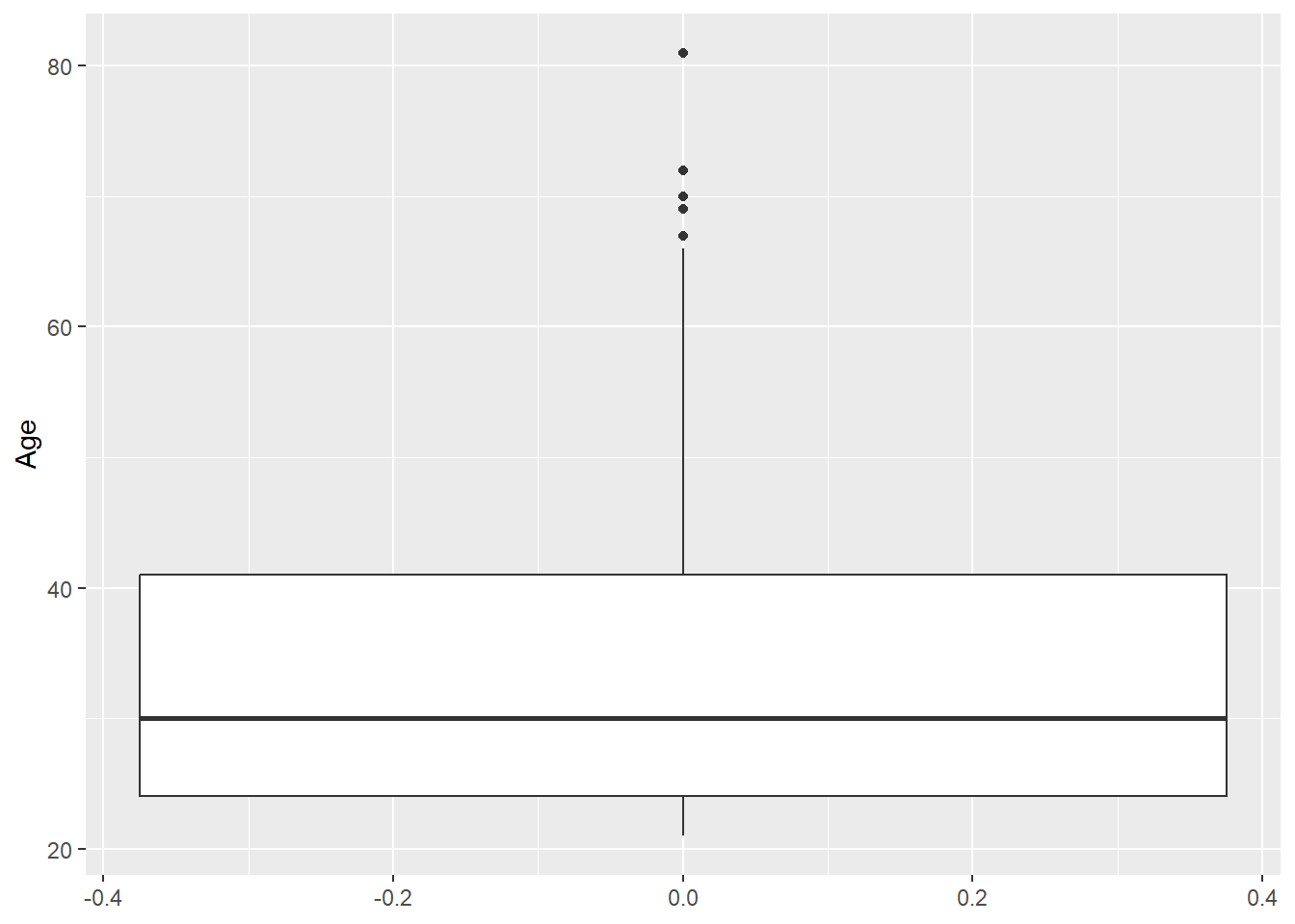
Odd: Some BloodPressure values are 0.
range(diabetes_clinical$BloodPressure, na.rm = TRUE)[1] 0 114diabetes_clinical %>%
ggplot(aes(y = BloodPressure, x = 1)) +
geom_violin() 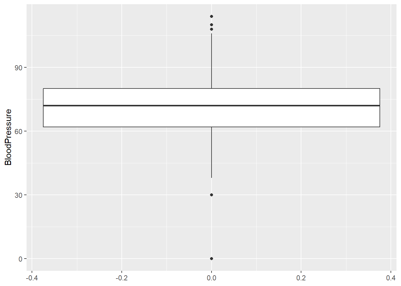
Odd: Some BMI values are 0.
range(diabetes_clinical$BMI, na.rm = TRUE)[1] 0.0 57.1diabetes_clinical %>%
ggplot(aes(y = BMI, x = 1)) +
geom_violin()Warning: Removed 3 rows containing non-finite outside the scale range
(`stat_ydensity()`).
range(diabetes_clinical$PhysicalActivity, na.rm = TRUE)[1] 19 177diabetes_clinical %>%
ggplot(aes(y = PhysicalActivity, x = 1)) +
geom_violin()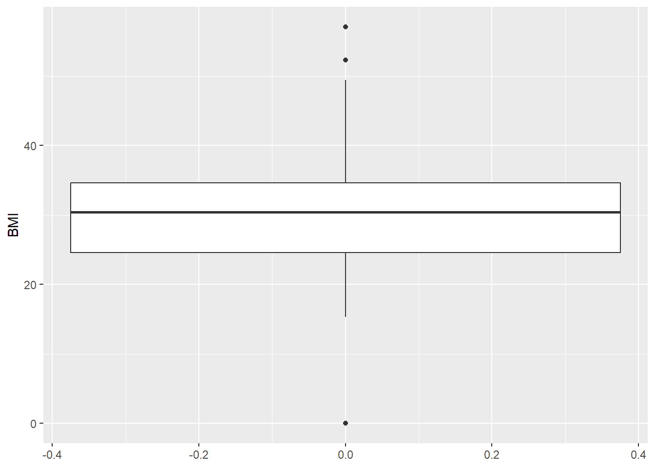
range(diabetes_clinical$Serum_ca2, na.rm = TRUE)[1] 8.7 10.2diabetes_clinical %>%
ggplot(aes(y = Serum_ca2, x = 1)) +
geom_violin()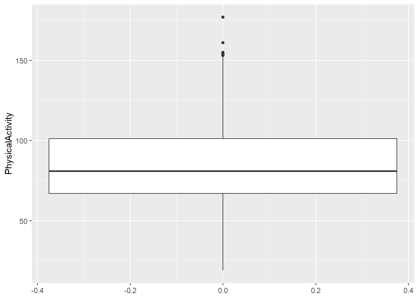
Clean up the data
Now that we have had a look at the data, it is time to correct fixable mistakes and remove observations that cannot be corrected.
Consider the following:
What should we do with the rows that contain NA’s? Do we remove them or keep them?
Which odd things in the data can we correct with confidence and which cannot?
Are there zeros in the data? Are they true zeros or errors?
Do you want to change any of the classes of the variables?
- Clean the data according to your considerations.
Hint
Have a look at ID, BloodPressure, BMI, Sex, and Diabetes.
My considerations:
When modelling, rows with NA’s in the variables we want to model should be removed as we cannot model on NAs. Since there are only NA’s in
AgeandBMI, the rows can be left until we need to do a model with these columns.The different spellings in
Sexshould be regularized so that there is only one spelling for each category. Since most rows have the first letter as capital letter and the remaining letter as lowercase we will use that.There are zeros in
BMIandBloodPressure. These are considered false zeros as is does not make sense that these variables have a value of 0.DiabetesandIDare changed to factor.
Check number of rows before cleaning.
nrow(diabetes_clinical)[1] 532Cleaning data according to considerations.
diabetes_clinical_clean <- diabetes_clinical %>%
  mutate(Sex = str_to_title(Sex),
         ID = factor(ID),
         Diabetes = factor(Diabetes)) %>%
  filter(BMI != 0, BloodPressure != 0)
Check the unique sexes now.
diabetes_clinical_clean$Sex %>% unique()[1] "Male" "Female"Check number of rows after cleaning.
nrow(diabetes_clinical_clean)[1] 490Meta Data
There is some metadata to accompany the dataset you have just cleaned in diabetes_meta_toy_messy.csv. This is a csv file, not an excel sheet, so you need to use the read_delim function to load it. Load in the dataset and inspect it.
6.2. Load the meta data set.
diabetes_meta <- read_delim('../data/diabetes_meta_toy_messy.csv')
head(diabetes_meta)
# A tibble: 6 × 3
ID Married Work
<dbl> <chr> <chr>
1 33879 Yes Self-employed
2 52800 Yes Private
3 16817 Yes Private
4 70676 Yes Self-employed
5 6319 No Public
6 71379 No Public 6.3. How many missing values (NA’s) are there in each column.
colSums(is.na(diabetes_meta)) ID Married Work
0 0 0 6.4. Check the distribution of each of the variables. Consider that the variables are of different classes. Do any of the distributions seam odd to you?
For the categorical variables:
table(diabetes_meta$Married)
  No  No   Yes Yes
183 3 345 1 table(diabetes_meta$Work)
      Private        Public       Retired Self-employed
          283           154             6            89
By investigating the unique values of the Married variable we see that some of the values have whitespace.
unique(diabetes_meta$Married)[1] "Yes" "No" "Yes " "No " - Clean the data according to your considerations.
My considerations:
The
Marriedvariable has whitespace in the some of the values. The values “Yes” and “Yes” will be interpreted as different values. We can confidently remove all the whitespaces in this variable.IDis changed to factor to match thediabetes_cleandataset.
Check number of rows before cleaning.
nrow(diabetes_meta)[1] 532diabetes_meta_clean <- diabetes_meta %>%
mutate(Married = str_trim(Married),
ID = factor(ID))Check the unique marital status now.
unique(diabetes_meta_clean$Married)[1] "Yes" "No" Check number of rows after cleaning.
nrow(diabetes_meta_clean)[1] 532Join the datasets
- Consider what variable the datasets should be joined on.
The joining variable must be the same type in both datasets.
- Join the datasets by the variable you selected above.
diabetes_join <- diabetes_clinical_clean %>%
left_join(diabetes_meta_clean, by = 'ID')- How many rows does the joined dataset have? Explain why.
Because we used left_join, only the IDs that are in diabetes_clinical_clean are kept.
nrow(diabetes_join)[1] 490- Export the joined dataset. Think about which directory you want to save the file in.
writexl::write_xlsx(diabetes_join, '../out/diabetes_join.xlsx')