library(tidyverse)
library(MASS)Exercise 5: Data Exercise in R
Introduction
In this exercise you will practice your newly acquired R skills on an example dataset.
For the data wrangling and statistical modelling we will be doing in this exercise, you will need the following R-packages: tidyverse, MASS.
- Make sure that these packages are installed and loaded into your R environment. You likely have the packages already installed and loaded (you used these in the previous exercises) try
sessionInfo()andrequire()(look up what these function do). If the packages are not there install them and library them as in the previous exercises.
Getting the Dataset
For this exercise, we’ll use the birthweight dataset from the package MASS. It contains the birthweight of infants and some information about the mother.
If you have your own data to work on, you can still follow the steps in the exercise where they apply.
To get it we have to load the package and then the data. We will also display the help so we can read some background info about the data and what the columns are:
N.B If it says <Promise> after birthwt in your global environment just click on it and the dataframe will be loaded properly.
If you have a dataset of your own you would like yo look at instead of the example data we provide here, you are very welcome to. You can again use read_excel() for excel sheets. For other formats, have a look at read.csv(), read.table(), read.delim(), etc. You can either google your way to an answer or ask one of the course instructors.
data(birthwt)
?birthwt #display help page- Now, check the class of the dataset. We’ll be using
tidyverseto do our anaylsis, so if it isn’t already a tibble, make it into one.
#Check class of data.
class(birthwt)
[1] "data.frame"#Convert into tibble.
birthwt <- as.tibble(birthwt)Warning: `as.tibble()` was deprecated in tibble 2.0.0.
ℹ Please use `as_tibble()` instead.
ℹ The signature and semantics have changed, see `?as_tibble`.#Check class of data to confirm that it is a tibble.
class(birthwt)[1] "tbl_df" "tbl" "data.frame"Exploratory Analysis
The Basics
Before performing any statistical analysis (modelling), it is necessary to have a good understanding of the data. Start by looking at:
- How many variables and observations are there in the data?
dim(birthwt) # rows, columns[1] 189 10- What was measured, i.e. what do each of the variables describe? You can rename variables via the
colnames()if you want to.
Run the command below to inspect the data. This can only be done to this dataset because it was loaded from a packages. Hence you will not be able to do this with your own data.
?birthwt- Which data types are the variables and does that make sense? Should you change the type of any variables? Hint: Think about types
factor, numerical, integer, character, etc.
str(birthwt)tibble [189 × 10] (S3: tbl_df/tbl/data.frame)
$ low : int [1:189] 0 0 0 0 0 0 0 0 0 0 ...
$ age : int [1:189] 19 33 20 21 18 21 22 17 29 26 ...
$ lwt : int [1:189] 182 155 105 108 107 124 118 103 123 113 ...
$ race : int [1:189] 2 3 1 1 1 3 1 3 1 1 ...
$ smoke: int [1:189] 0 0 1 1 1 0 0 0 1 1 ...
$ ptl : int [1:189] 0 0 0 0 0 0 0 0 0 0 ...
$ ht : int [1:189] 0 0 0 0 0 0 0 0 0 0 ...
$ ui : int [1:189] 1 0 0 1 1 0 0 0 0 0 ...
$ ftv : int [1:189] 0 3 1 2 0 0 1 1 1 0 ...
$ bwt : int [1:189] 2523 2551 2557 2594 2600 2622 2637 2637 2663 2665 ...Change the appropriate variables to factor.
birthwt <- birthwt %>%
  mutate(low = factor(low),
         race = factor(race),
         smoke = factor(smoke),
         ht = factor(ht),
         ui = factor(ui)
)- What is our response/outcome variable(s)? There can be several.
bwt (birth weight) and low (the indicator of birth weight less than 2.5 kg).
- Is the (categorical) outcome variable balanced?
birthwt$low %>% table().
0 1
130 59 No, the categorical outsome variable (low) is not very balanced.
- Are there any missing values (
NA), if yes and how many? Google how to check this if you don’t know.
birthwt %>% is.na() %>% colSums() low age lwt race smoke ptl ht ui ftv bwt
0 0 0 0 0 0 0 0 0 0 No, there are no NA values in any of the columns.
Diving into the data
Numeric variables
Some of the measured variables in our data are numeric, i.e. continuous. For these do:
- Calculate summary statistics (mean, median, min, max) with
summaryfunction.
birthwt %>%
  dplyr::select(age, lwt, ptl, ftv, bwt) %>%
  summary()
age lwt ptl ftv
Min. :14.00 Min. : 80.0 Min. :0.0000 Min. :0.0000
1st Qu.:19.00 1st Qu.:110.0 1st Qu.:0.0000 1st Qu.:0.0000
Median :23.00 Median :121.0 Median :0.0000 Median :0.0000
Mean :23.24 Mean :129.8 Mean :0.1958 Mean :0.7937
3rd Qu.:26.00 3rd Qu.:140.0 3rd Qu.:0.0000 3rd Qu.:1.0000
Max. :45.00 Max. :250.0 Max. :3.0000 Max. :6.0000
bwt
Min. : 709
1st Qu.:2414
Median :2977
Mean :2945
3rd Qu.:3487
Max. :4990 - Calculate standard deviation with
summarizefunction.
birthwt %>%
  dplyr::select(age, lwt, ptl, ftv, bwt) %>% # Specify select function from the dplyr package.
  summarize(age_sd = sd(age),
            lwt_sd = sd(lwt),
            ptl_sd = sd(ptl),
            ftv_sd = sd(ftv),
            bwt_sd = sd(bwt)
  )
# A tibble: 1 × 5
age_sd lwt_sd ptl_sd ftv_sd bwt_sd
<dbl> <dbl> <dbl> <dbl> <dbl>
1 5.30 30.6 0.493 1.06 729.- Create a density for a continuous variable using
ggplot2. Do this for all the numeric variables (age,lwt,ptl,ftv,bwt).
ggplot(birthwt,
       aes(x = age)) +
  geom_density() +
  theme_bw()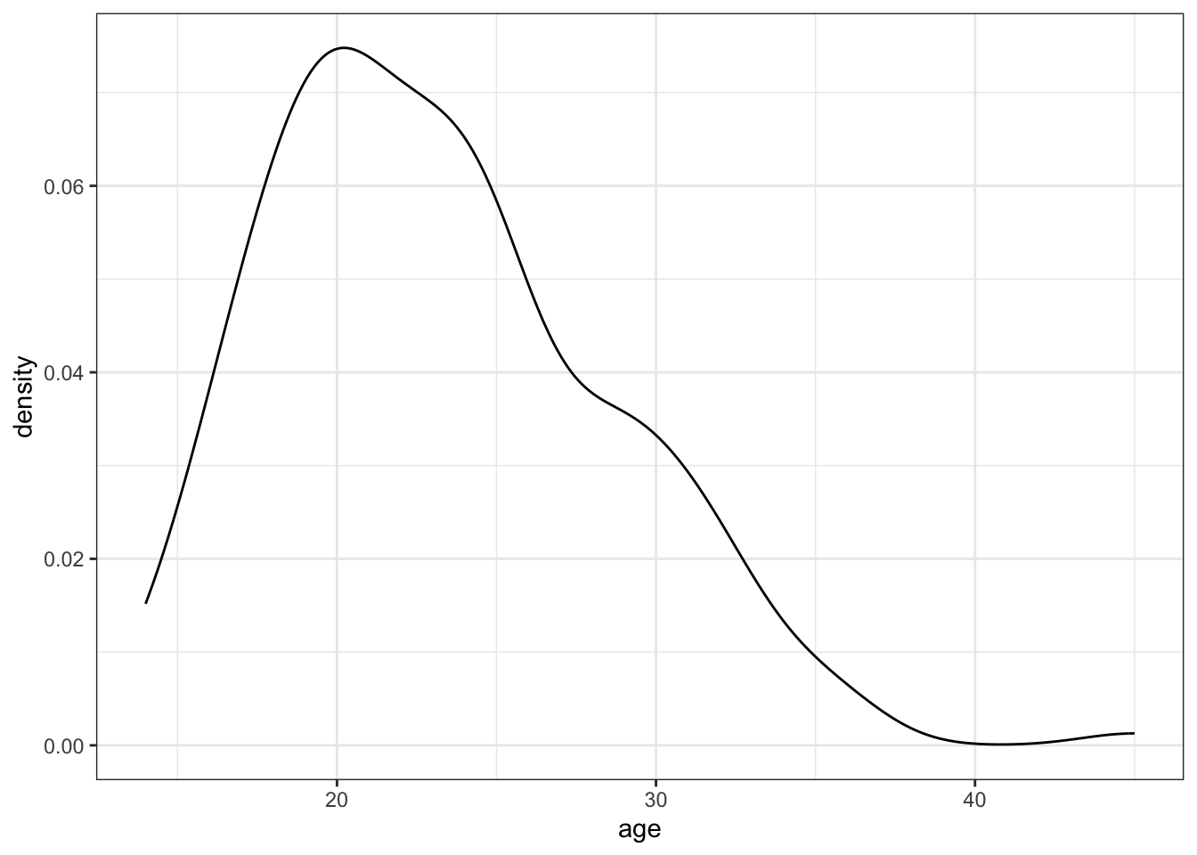
- Look at the distribution of mothers’ age (
age). Are mothers older than 40 possible outliers in this dataset?
Make a small summary table (min, max, mean, sd and mean+(3*sd)) that helps you decide whether you want to exclude ages > 40 before modelling. Count how many observations are > 40.
Then createbirthwt_subset(either filtered or unfiltered) with the variables we will use going forward:age,lwt,smoke,ui,low,bwt.
#ggplot(birthwt, aes(y = age)) +
#  geom_boxplot() +
#  theme_bw()

birthwt %>%
  summarise(
    min_age = min(age),
    max_age = max(age),
    mean_age = mean(age),
    sd_age = sd(age),
    cutpoint = mean(age)+(3*sd(age))
  )
# A tibble: 1 × 5
min_age max_age mean_age sd_age cutpoint
<int> <int> <dbl> <dbl> <dbl>
1 14 45 23.2 5.30 39.1birthwt %>%
summarise(n_over_40 = sum(age > 40),
prop_over_40 = mean(age > 40))# A tibble: 1 × 2
n_over_40 prop_over_40
<int> <dbl>
1 1 0.00529birthwt_subset <- birthwt %>%
filter(age <= 40) %>%
dplyr::select(age, lwt, smoke, ui, ui, low, bwt)- Now make the boxplot of age according to birth weigh categories. Pick custom colors for your plot. Use birthwt_subset from now on.
TipHint
Look into scale_fill_manual()
ggplot(birthwt_subset,
       aes(y = age,
           x = low,
           fill = low)) +
  geom_boxplot() +
  scale_fill_manual(values = c('black', 'grey')) +
theme_bw() 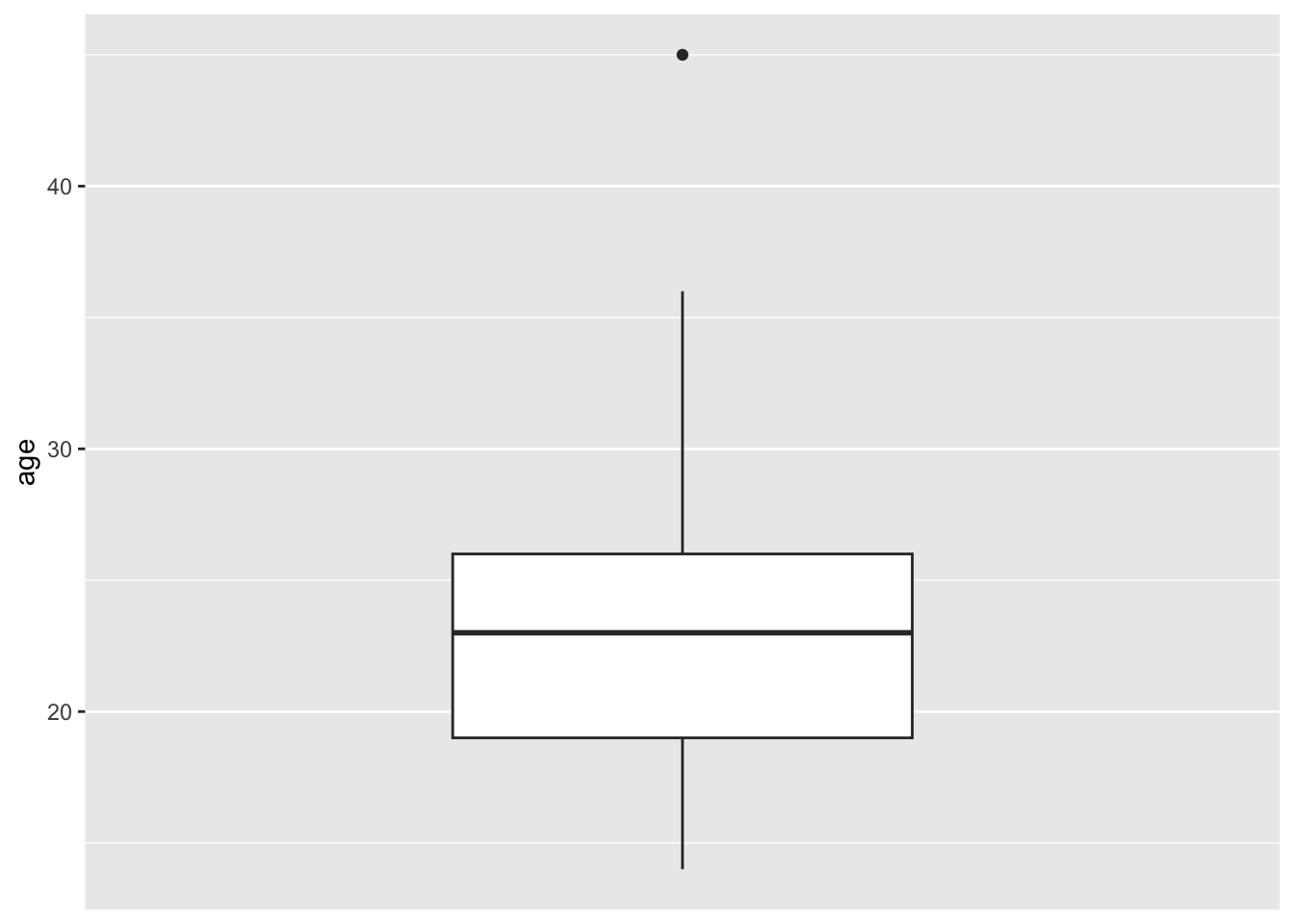
Categorical variables
- Some variables in
birthwtare categorical, but may be coded as 0/1 and therefore read in as numeric. If you haven’t changed their datatype to factor yet, do so now. Then make a stacked bar plot forsmokeshowing counts, split by the outcome variablelowby mappingfill = low(using two colors as above).
ggplot(birthwt_subset,
       aes(x = smoke,
           fill = low)) +
  geom_bar() +
  scale_fill_manual(values = c('black', 'grey')) +
theme_bw() 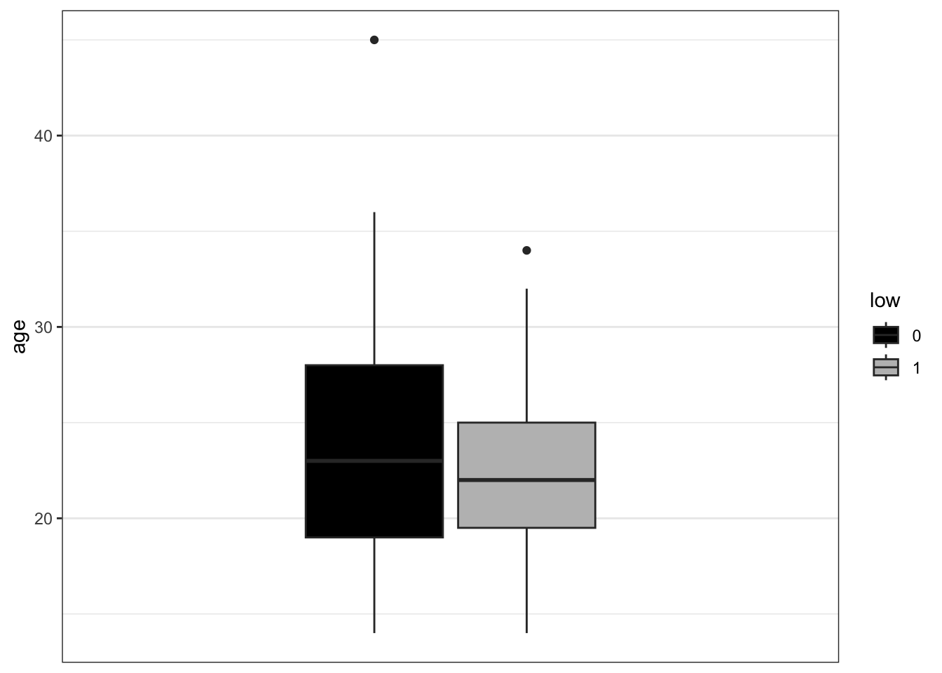
- Remake the bar plot for
smoke, but this time split eachsmokebar by the outcome variablelowby mapping fill = low, using two colors (as you did for the boxplots). Then addposition = "dodge"to geom_bar() and remake the plot. Compared to the default (stacked) bar plot, what changes when you use “dodge”?
ggplot(birthwt_subset,
       aes(x = smoke,
           fill = low)) +
  geom_bar(position = 'dodge') +
  scale_fill_manual(values = c('black', 'grey')) +
theme_bw() 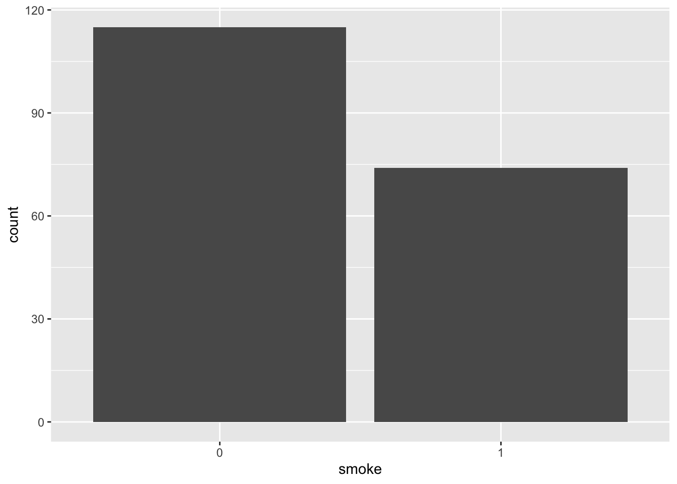
What information do the different barplots show? Compare to the counts you get from the smoke column when you group the dataframe by the outcome variable.
- Create a tidy summary table using one pipeline. Starting from
birthwt, do all of the following in a single%>%chain:- Create a new variable
lwt_kgthat convertslwtfrom pounds to kilograms (1 lb = 0.453592 kg) - Group by
smokeandlow - Compute:
n(number of observations)- mean and sd of
bwt - mean of
lwt_kg
- Arrange the output so the largest mean birth weight is on top
- Create a new variable
birthwt_summary <- birthwt_subset %>%
  mutate(lwt_kg = lwt * 0.453592) %>%
  group_by(smoke, low) %>%
  summarise(
    n = n(),
    mean_bwt = mean(bwt),
    sd_bwt = sd(bwt),
    mean_lwt_kg = mean(lwt_kg),
    .groups = "drop"
  ) %>%
  arrange(desc(mean_bwt))

birthwt_summary
# A tibble: 4 × 6
smoke low n mean_bwt sd_bwt mean_lwt_kg
<fct> <fct> <int> <dbl> <dbl> <dbl>
1 0 0 85 3376. 472. 61.1
2 1 0 44 3201. 408. 59.4
3 1 1 30 2143. 400. 56.3
4 0 1 29 2050. 383. 54.5- Make one “publication-ish” plot: a boxplot of birth weight (
bwt) by smoking status (smoke), colored by the combined groups of birthweight category (low) and presence of uterine irritability (ui).
To make the legend readable, first create labeled versions oflowandui, then combine them into an interaction variable (e.g.low_ui). Your plot should include:
- a clear title and axis labels
- a clean theme
- custom fill colors
- a clear legend title (e.g. “Birthweight group + HT”)
birthwt_subset <- birthwt_subset %>%
  mutate(
    low_lab = factor(low, levels = c(0, 1),
                     labels = c("Normal BW", "Low BW")),
    ui_lab  = factor(ui,  levels = c(0, 1),
                     labels = c("No UI", " Yes UI")),
    low_ui  = interaction(low_lab, ui_lab, sep = " + ", drop = TRUE)
  )

p_bwt_smoke <- ggplot(birthwt_subset,
                      aes(x = smoke,
                          y = bwt,
                          fill = low_ui)) +
  geom_boxplot(outlier.alpha = 0.6) +
  scale_fill_manual(values = c("black",  "blue", "grey", "lightblue"),
                    name = "Low BW : UI") +
  labs(
    title = "Birth weight by smoking status",
    x = "Mother smokes",
    y = "Birth weight (g)"
  ) +
  theme_bw()

p_bwt_smoke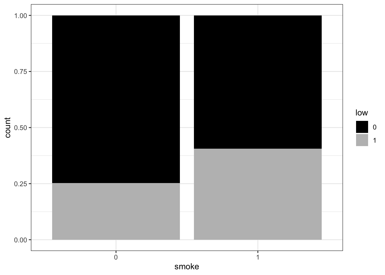
Modelling
You now have a prepared dataset on which we can do some modelling.
Regression Model 1
In the Applied statistics session you’ve tried out an analysis with one way ANOVA, where you compared the effect of categorical variables (skin type) on the outcome (gene counts).
We’ll do something similar here but instead we will use the numerical variables as predictors and the measured birthweight as the (numerical) outcome. This is what is known as linear regression.
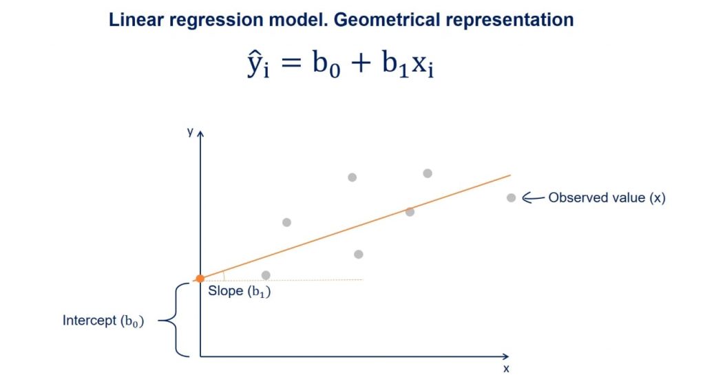
We can also do this with lm() and follow the same syntax as before:
model1 <- lm(resp ~ pred1, data=name_of_dataset)Simply, if the outcome variable we are interested in is continuous, then lm() will functionally be doing a linear regression. If the outcome is categorical, it will be performing ANOVA (which if you only have two groups is effectively a t-test). Have a look at this video if you want to understand why you can do a t-test / ANOVA with a linear model.
- Now, pick one of your numeric variables and use it to model the (numeric/continuous) outcome.
model1_lwt <- lm(bwt ~ lwt, data = birthwt_subset)- Investigate the model you have made by writing its name, i.e.
model1_lwt- What does this mean? Compare to the linear model illustration above.
At the intercept the lwt (mother’s weight in pounds) is 0 (very unrealistic) the bwt is 2369.624 grams. For each pound that a mother weighs more, the btw is 4.429 grams more.
- We’ll now make a plot of your model to help us better visualize what has happened. Make a scatter plot with your predictor variable on the x-axis and the outcome variable on the y-axis.
ggplot(birthwt_subset,
       aes(x = lwt,
           y = bwt)) +
  geom_point()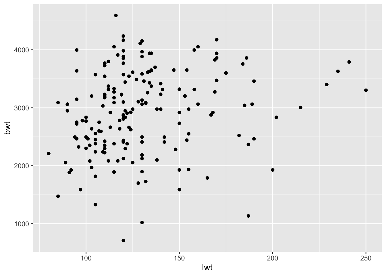
- Now add the regression line to the plot by using the code below. For the slope and intercept, enter the values you found when you inspected the model. Does this look like a good fit?
ggplot(birthwt_subset,
       aes(x = lwt,
           y = bwt)) +
  geom_point() +
  geom_abline(slope = model1_lwt$coefficients["lwt"],
              intercept = model1_lwt$coefficients["(Intercept)"],
              color = 'red')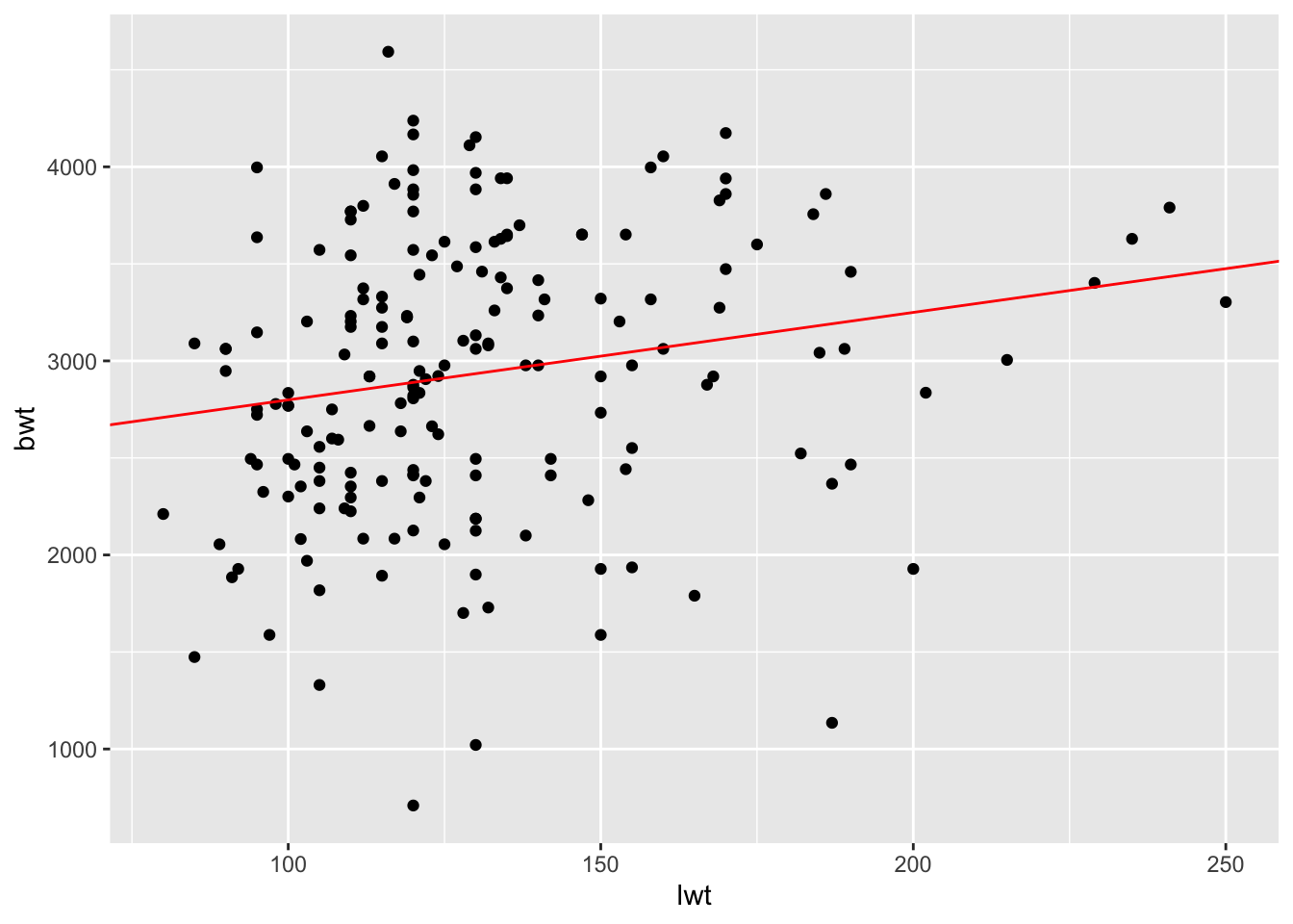
- Instead of the
geom_abline(), trygeom_smooth()which provides you with a confidence interval in addition to the regression line. Look at the help for this geom (or google) to figure out what argument it needs to work!
ggplot(birthwt_subset,
       aes(x = lwt,
           y = bwt)) +
  geom_point() +
  geom_smooth(method = "lm",
              formula = y ~ x,
              color = 'red')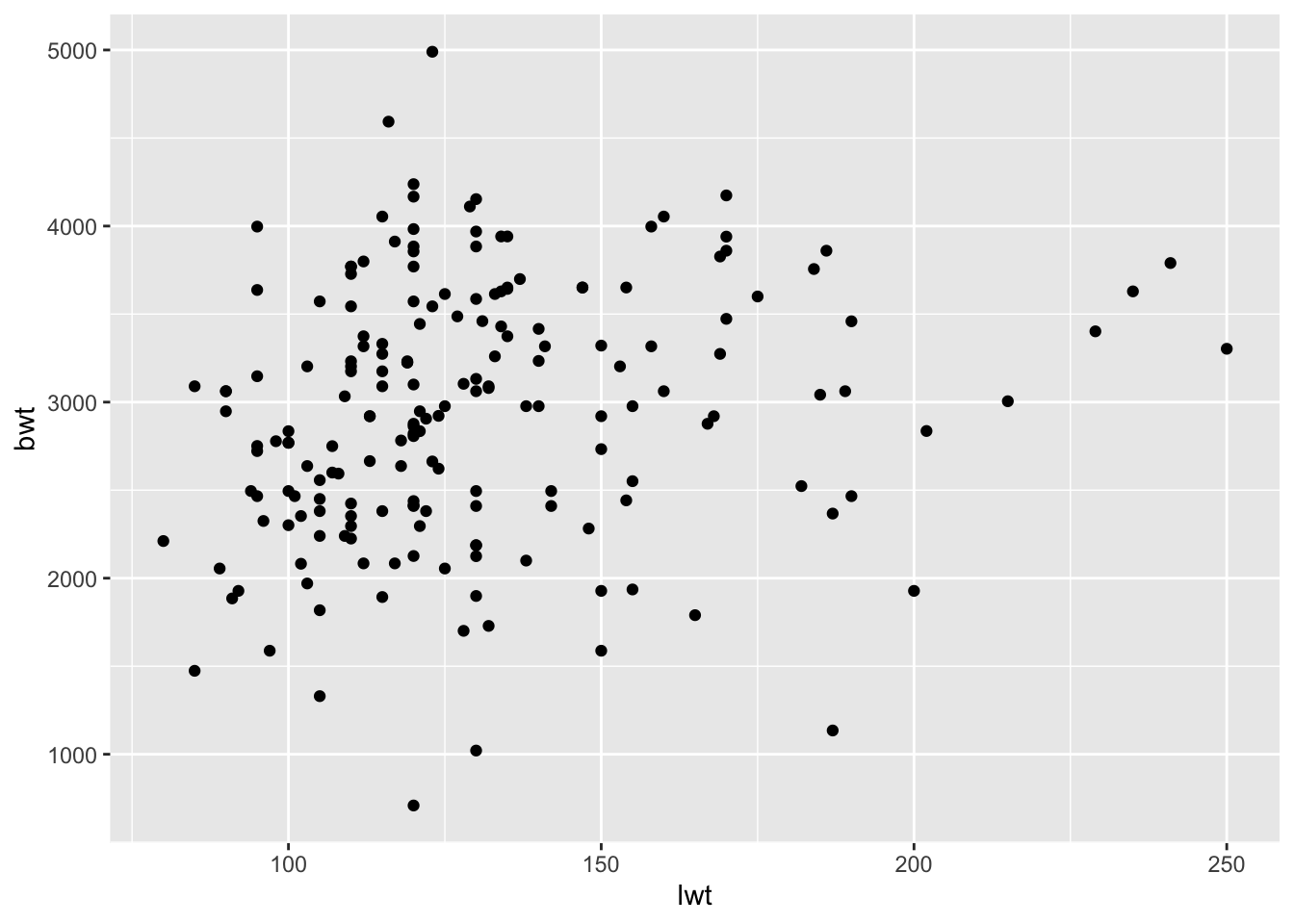
- Repeat the process with the other numeric variable you picked.
model1_age <- lm(bwt ~ age, data = birthwt_subset)
model1_age
Call:
lm(formula = bwt ~ age, data = birthwt_subset)

Coefficients:
(Intercept)          age
2833.273 4.344 - Inspect your model in more detail with
summary(). Look at the output, what additional information do you get about the model. Pay attention to theResidual standard error (RSE)andAdjusted R-squared (R2adj)at the bottom of the output. We would likeRSEto be as small as possible (goes towards 0 when model improves) while we would like theR2adjto be large (goes towards 1 when model improves).
summary(model1_lwt)
Call:
lm(formula = bwt ~ lwt, data = birthwt_subset)

Residuals:
     Min       1Q   Median       3Q      Max
-2180.28  -487.09     7.12   488.39  1721.76

Coefficients:
            Estimate Std. Error t value Pr(>|t|)
(Intercept) 2348.077    224.025  10.481  < 2e-16 ***
lwt            4.510      1.679   2.686  0.00789 **
---
Signif. codes:  0 '***' 0.001 '**' 0.01 '*' 0.05 '.' 0.1 ' ' 1

Residual standard error: 704 on 186 degrees of freedom
Multiple R-squared:  0.03733,   Adjusted R-squared:  0.03215
F-statistic: 7.213 on 1 and 186 DF, p-value: 0.007894summary(model1_age)
Call:
lm(formula = bwt ~ age, data = birthwt_subset)

Residuals:
     Min       1Q   Median       3Q      Max
-2245.89  -511.24    26.45   540.09  1655.48

Coefficients:
            Estimate Std. Error t value Pr(>|t|)
(Intercept) 2833.273    244.954   11.57   <2e-16 ***
age            4.344     10.349    0.42    0.675
---
Signif. codes:  0 '***' 0.001 '**' 0.01 '*' 0.05 '.' 0.1 ' ' 1

Residual standard error: 717.2 on 186 degrees of freedom
Multiple R-squared:  0.0009461, Adjusted R-squared:  -0.004425
F-statistic: 0.1761 on 1 and 186 DF,  p-value: 0.6752
Sometimes the variables we have measured are not good at explaining the outcome and we have to accept that.
N.B if you want to understand the output of a linear regression summary in greater detail have a look here.
Regression Model 2
- Remake your model (call it
model2) but this time add an additional explanatory variable to the model in addition tolwt. This should be the categorical variable you selected to be in your subset. Does adding this second exploratory variable improve the metricsRSEand/orR2adj?
TipHint
model2 <- lm(resp ~ pred1 + pred2, data=name_of_dataset)model2 <- lm(bwt ~ lwt + ui, data=birthwt_subset)
model2
Call:
lm(formula = bwt ~ lwt + ui, data = birthwt_subset)

Coefficients:
(Intercept)          lwt          ui1
2546.820 3.578 -521.906 summary(model2)
Call:
lm(formula = bwt ~ lwt + ui, data = birthwt_subset)

Residuals:
     Min       1Q   Median       3Q      Max
-2080.92  -467.27   -24.11   551.40  1631.12

Coefficients:
            Estimate Std. Error t value Pr(>|t|)
(Intercept) 2546.820    223.341  11.403  < 2e-16 ***
lwt            3.578      1.644   2.176 0.030827 *
ui1         -521.906    141.219  -3.696 0.000289 ***
---
Signif. codes:  0 '***' 0.001 '**' 0.01 '*' 0.05 '.' 0.1 ' ' 1

Residual standard error: 681.2 on 185 degrees of freedom
Multiple R-squared:  0.1035,    Adjusted R-squared:  0.09382
F-statistic: 10.68 on 2 and 185 DF, p-value: 4.075e-05- Find the 95% confidence intervals for model2, by using the
confint()function. If you are not familiar with confidence intervals, have a look here.
confint(model2) 2.5 % 97.5 %
(Intercept) 2106.1981178 2987.442789
lwt 0.3339242 6.822238
ui1 -800.5124113 -243.298849- Make a scatterplot of birth weight (bwt) vs mother’s weight (lwt). Color the points by uterine irritability (ui), and add a linear regression trend line using geom_smooth(method = “lm”).
ggplot(birthwt_subset,
       aes(x = lwt,
           y = bwt,
           fill = ui,
           color = ui)) +
  geom_point() +
  geom_smooth(method = "lm",
              formula = y ~ x,
              color = 'red')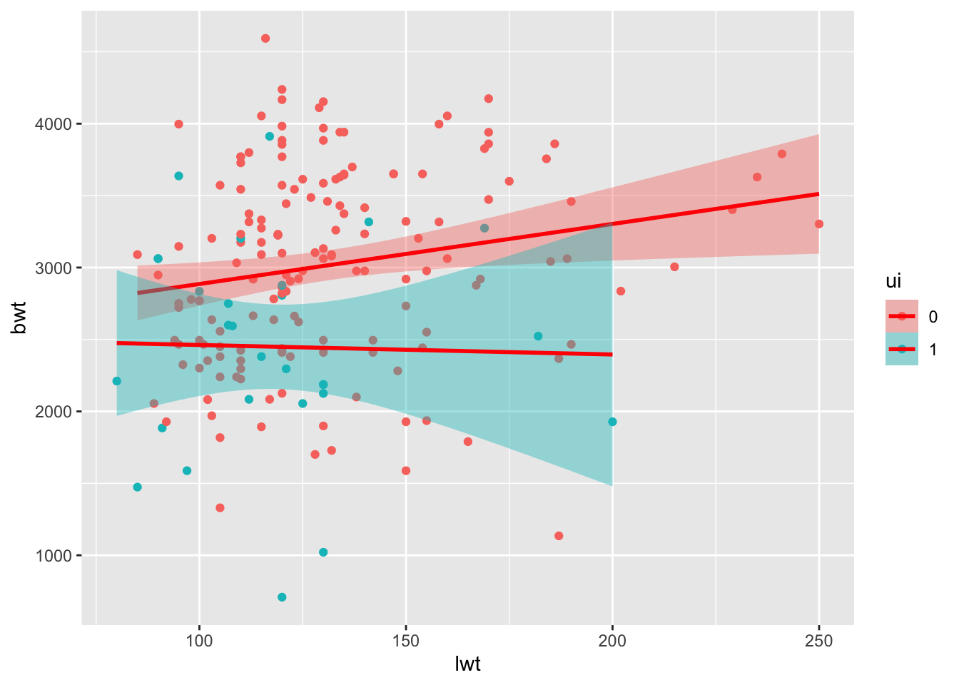
- Try the following commands (or a variation of it, depending on which variables you have included in model2), and see if you can figure out what the outcome means.
newData <- data.frame(lwt=100, age = 50, smoke=as.factor(1))
newData
predict(model2, newData)
predict(model2, newData, interval="prediction")
Bonus Exercise - ANOVA
Now, we will instead look at the two categorical variables you picked. Make a model of the outcome variable depending on one the categorical variable
- Pick one of the two categorical variables and use it to model the (numeric) outcome, just as during the Applied Stats session:
model3 <- lm(bwt ~ smoke, data=birthwt_subset)- inspect the output by calling
summary()on the model
summary(model3)You can have a look at this website to help you understand the output of summary.
Short detour: The meaning of the intercept in an ANOVA
The intercept is the estimate of the outcome variable that you would get when all explanatory variables are 0.
So if we have the model lm(bwt ~ smoke, data = birthData) and smoke is coded as 0 for non-smokers and 1 for smokers, the intercept is the estimate birthweight of a baby of a non-smoker. It will be significant because it is significantly different from 0, but that doesn’t mean much since we would usually expect babies to weight more than 0.
You can now make some other models, including several predictors and see what you get.