#install.packages("tidyverse")
#install.packages("readxl")
#install.packages("emmeans")
library(tidyverse)
library(readxl)
library(emmeans)Exercise 4, Part 1: Applied Statistics in R - Solutions
You can download the exercise4_PART1_solutions.qmd file and explore it in your RStudio. Just clink on the file link, download from GitHub and open the file in your local RStudio.
Structure of a biostatistical analysis in R
The very basic structure of an R script doing a classical statistical analysis is as follows:
- Load packages that you will be using.
- Read the dataset to be analyzed. Possibly also do some data cleaning and manipulation.
- Visualize the dataset by graphics and other descriptive statistics.
- Fit and validate a statistical model.
- Hypothesis testing. Possibly also post hoc testing.
Of course there are variants of this set-up, and in practice there will often be some iterations of the steps.
In this manuscript we will exemplify the proposed steps in the analysis of a simple dataset:
- In our current scenario, you are a researcher investigating psoriasis, an inflammatory skin disease. You have data on the expression of a number genes that are suspected to have something to do with the disease, but you cannot be sure until you perform some formal statistical analysis.
- This is a great example where R skills would come very handy!
- You will investigate your gene of special interest GeneD (a hypothetical gene in this case).
- You decide that your analysis approach will be one-way ANOVA of the expression of GeneD against the skin type in psoriasis patients.
Load packages
We will use ggplot2 to make plots, and to be prepared for data manipulations, we simply load this together with the rest of the tidyverse.
The psoriasis data are provided in an Excel sheet, so we also load readxl. Finally, we will use the package emmeans to make post hoc tests.
Remember that you should install the wanted packages before they can be used (but you only need to install the packages once!).
Thus,
Now, we are done preparing for our analyses. Next, we will look specifically at the possible association between GeneD expression and psoriasis. Finally, we conclude with a brief outlook on other statistical models in R.
Please refer to the ‘STATS CHEAT SHEET’ provided in the slides for hints as well as other cheat sheets provided in other sessions where necessary.
Example: Analysis of variance
Step 1: Data
Psoriasis is an immune-mediated disease that affects the skin. You, as a researcher, carried out a micro-array experiment with skin from 37 people in order to examine a potential association between the disease and a certain gene (GeneD). For each of the 37 samples the gene expression was measured. Fifteen skin samples were from psoriasis patients and from a part of the body affected by the disease (psor); 15 samples were from psoriasis patients but from a part of the body not affected by the disease (psne); and 7 skin samples were from healthy people (control).
The data are saved in the file psoriasis.xlsx. At first the variable type is stored as a character variable, we change it to a factor (and check that indeed there are 15, 15 and 7 patients in the three groups).
psoriasisData <- read_excel("../../Data/psoriasis.xlsx")

# Dataset1
psorData  <- select(psoriasisData, type, GeneD)

# Dataset2
psorDataG <- select(psoriasisData, -GeneD)


psorData <- mutate(psorData, type = factor(type))
count(psorData, type)
# A tibble: 3 × 2
type n
<fct> <int>
1 healthy 7
2 psne 15
3 psor 15Step 2: Descriptive plots and statistics
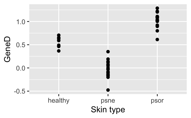
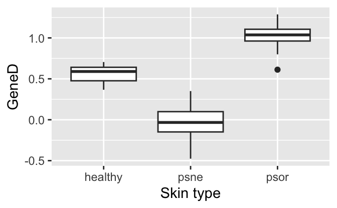
To get an impression of the data, we make two plots and compute group-wise means and standard deviations.
ggplot(psorData, aes(x=type, y=GeneD)) +
  geom_point() +
  labs(x="Skin type", y="GeneD")

ggplot(psorData, aes(x=type, y=GeneD)) +
  geom_boxplot() +
  labs(x="Skin type", y="GeneD")

psorData %>%
  group_by(type) %>%
  summarise(avg=mean(GeneD), median=median(GeneD), sd=sd(GeneD))
# A tibble: 3 × 4
type avg median sd
<fct> <dbl> <dbl> <dbl>
1 healthy 0.557 0.590 0.121
2 psne -0.0292 -0.0331 0.197
3 psor 1.03 1.04 0.171

Step 3: Fit of oneway ANOVA, model validation
The scientific question is whether the gene expression level of GeneD differs between the three types/groups. Thus, the natural type of analysis is a oneway analysis of variance (ANOVA). The oneway ANOVA is fitted with a function in R. It is a good approach to assign a name (below oneway) to the object with the fitted model. This object contains all relevant information and may be used for subsequent analysis. Note that we need to logarithmic transform the response as intensities are often on a multiplicative scale.
oneway <- lm(log(GeneD) ~ type, data=psorData)
oneway
Call:
lm(formula = log(GeneD) ~ type, data = psorData)

Coefficients:
(Intercept)     typepsne     typepsor
    -0.6079      -1.4693       0.6198
Step 4: Hypothesis test + Post hoc tests
It is standard to carry out an \(F\)-test for the overall effect of the explanatory (i.e. independent) variable. To be precise, the hypothesis is that the expected values are the same in all groups. The most easy way to do this test is to use ???. Hint: The option test="F" is needed to get the \(F\)-test using that function:
drop1(oneway,test="F")Single term deletions
Model:
log(GeneD) ~ type
Df Sum of Sq RSS AIC F value Pr(>F)
<none> 3.345 -53.492
type 2 18.707 22.052 -4.686 69.907 5.779e-11 ***
---
Signif. codes: 0 '***' 0.001 '**' 0.01 '*' 0.05 '.' 0.1 ' ' 1Thus, the overall test for homogeneity between the groups show that the groups are not all the same. But it might be that the gene expression in two of the three groups, say, are not significantly different. To investigate that we do post hoc testing. This is nicely done within the framework of estimated marginal means using the emmeans package. Here emmeans makes the estimated marginal means (that is the predicted gene expression of GeneD on the log scale), and the pairs() command provide post hoc pairwise comparisons (package automatically adjusts for multiple comparisons using the default tukey method):
emmeans(oneway,~type) type emmean SE df lower.CL upper.CL
healthy -0.6079 0.1383 25 -0.893 -0.323
psne -2.0772 0.1493 25 -2.385 -1.770
psor 0.0119 0.0944 25 -0.183 0.206
Results are given on the log (not the response) scale.
Confidence level used: 0.95 pairs(emmeans(oneway,~type)) contrast estimate SE df t.ratio p.value
healthy - psne 1.47 0.204 25 7.220 <.0001
healthy - psor -0.62 0.167 25 -3.702 0.0029
psne - psor -2.09 0.177 25 -11.823 <.0001
Results are given on the log (not the response) scale.
P value adjustment: tukey method for comparing a family of 3 estimates GeneD expression levels are significantly different between all three groups of skin samples when we perform pairwise comparisons across the three groups ([1]healthy - psne, [2]healthy - psor and [3]psne - psor; all p-values < 0.05).
Outlook: Other analyses
The lm function is used for linear models, that is, models where data points are assumed to be independent with a Gaussian (i.e. normal) distribution (and typically also with the same variance). Obviously, these models are not always appropriate, and there exists functions for many, many more situations and data types. Here, we just mention a few functions corresponding to common data types and statistical problems.
glm: For independent, but non-Gaussian data. Examples are binary outcomes (logistic regression) and outcomes that are counts (Poisson regression). glm is short for generalized linear models, and theglmfunction is part of the base installation of R.lmerandglmer: For data with dependence structures that can be described by random effects, e.g., block designs. lme is short for linear mixed effects (Gaussian data), glmer is short for generalized linear mixed effects (binary or count data). Both functions are part of the lme4 package.nls: For non-linear regression, e.g., dose-response analysis. nls is short for non-linear least squares. The function is included in the base installation of R.
The functions mentioned above are used in a similar way as lm: a model is fitted with the function in question, and the model object subsequently examined with respect to model validation, estimation, computation of confidence limits, hypothesis tests, prediction, etc. with functions summary, confint, drop1, emmeans, pairs as mostly indicated above.