1+3[1] 4Want to code along? Go to the Data tab of the website and press the DOWNLOAD PRESENTATIONS button. This is presentation 1.
Quarto is an open-source publishing suite - a tool-suite that supports workflows for reproducible scholarly writing and publishing.
Quarto documents often begin with a YAML header demarcated by three dashes (---) which specifies things about the document. This includes what type of documents to render (compile) to e.g. HTML, PDF, WORD and whether it should be published to a website project. You can also add information on project title, author, default editor, etc.
Quarto works with markup language. A markup language is a text-coding system which specifies the structure and formatting of a document and the relationships among its parts. Markup languages control how the content of a document is displayed.
Pandoc Markdown is the markup language utilized by Quarto - another classic example of a markup language is LaTeX.
Let´s see how the pandoc Pandoc Markdown works:
Headers are marked with hashtags. More hashtags equals smaller title.
This is normal text. Yes, it is larger than the smallest header. A Quarto document works similarly to a Word document where you can select tools from the toolbar to write in bold or italic and insert thing like a table:
| My friends | Their favorite drink | Their favorite food |
|---|---|---|
| Michael | Beer | Burger |
| Jane | Wine | Lasagne |
| Robert | Water | Salad |
… a picture:

We can also make a list of things we like:
Coffee
Cake
Water
Fruit
There are two modes of Quarto: Source and Visual. In the left part of the panel you can change between the two modes.
Some features can only be added when you are in Source mode. E.g write blue text is coded like this in the source code [write blue text]{style="color:blue"}.
Note: Sometimes, if you are stuck in Quarto’s Visual mode, it’s worth switching between Source and Visual modes to reset things.
Code chunks are where the code is added to the document.
Click the green button +c and a grey code chunk will appear with '{r}' in the beginning. This means that it is an R code chunk. It is also possible to insert code chunks of other coding language.
For executing the code, press the Run button in the top right of the chunk to evaluate the code.
some executable code in an R code chunk.
1+3[1] 4Below is a code chunk with a comment. A comment is a line that starts with a hashtag. Comments can be useful in longer code chunks and will often describe the code.
# This is a comment. Here I can write whatever I want because it is in hashtags. You can add comments above or to the right of the code. This will not influence the executing of the code.
# Place a comment here
1+3 # or place a comment here
[1] 4Control whether code is executed.
eval=FALSE will not execute the code and eval=TRUE will execute the code in the compiled document.
The code is shown, but the result is not shown ({r, echo=TRUE, eval=FALSE}):
1+3Show or hide code. echo=FALSE will hide the code and echo=TRUE will show the code. Default is TRUE.
The code is not shown, but the result is shown ({r, echo=FALSE, eval=TRUE}):
[1] 4Control messages, warnings and errors. Maybe you have a code chunk that you know will produce one of the three and you often don’t want to see it in the compiled document.
log(-1)Warning in log(-1): NaNs produced[1] NaNWarning and error is not printed ({r, message=FALSE, warning=FALSE, error=TRUE}):
log(-1)[1] NaNstop("Intentional error for teaching.")Error:
! Intentional error for teaching.If an error occurs unexpectedly during rendering, Quarto will halt the render, so errors should be fixed (or intentionally demonstrated using error: true / tryCatch()).
N.B! It is not a good idea to hide these statements (especially the errors) before you know what they are.
In the panel there is a blue arrow and the word Render. Open the rendered html file in your browser and admire your work.
Now let’s get back to coding!
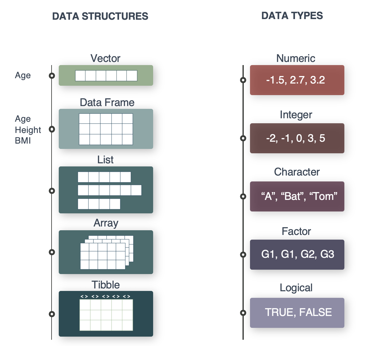
In the example below we will make two vectors into a tibble. Tibbles are the R object types you will mainly be working with in this course. We will try to convert between data types and structures using the collection of ‘as.’ functions.
A vector of characters
people <- c("Anders", "Diana", "Tugce", "Henrike", "Chelsea", "Valentina", "Thilde", "Helene")
people
[1] "Anders" "Diana" "Tugce" "Henrike" "Chelsea" "Valentina"
[7] "Thilde" "Helene" A vector of numeric values
joined_year <- c(2019, 2020, 2020, 2021, 2023, 2022, 2020, 2024)
joined_year
[1] 2019 2020 2020 2021 2023 2022 2020 2024Access data type or structure with the class() function
class(people)[1] "character"class(joined_year)[1] "numeric"Convert joined_year to character values
joined_year <- as.character(joined_year)
joined_year
[1] "2019" "2020" "2020" "2021" "2023" "2022" "2020" "2024"class(joined_year)[1] "character"Convert joined_year back to numeric values
joined_year <- as.numeric(joined_year)
joined_year
[1] 2019 2020 2020 2021 2023 2022 2020 2024Convert classes with the ‘as.’ functions
# We will try to convert between data types and structures using the collection of 'as.' functions.

# as.numeric()
# as.integer()
# as.character()
# as.factor()
# ...
Let’s make a tibble from two vectors
library(tidyverse) # run each time you start R── Attaching core tidyverse packages ──────────────────────── tidyverse 2.0.0 ──
✔ dplyr 1.2.1 ✔ readr 2.2.0
✔ forcats 1.0.1 ✔ stringr 1.6.0
✔ ggplot2 4.0.2 ✔ tibble 3.3.1
✔ lubridate 1.9.5 ✔ tidyr 1.3.2
✔ purrr 1.2.1
── Conflicts ────────────────────────────────────────── tidyverse_conflicts() ──
✖ dplyr::filter() masks stats::filter()
✖ dplyr::lag() masks stats::lag()
ℹ Use the conflicted package (<http://conflicted.r-lib.org/>) to force all conflicts to become errorsmy_data <- tibble(name = people,
joined_year = joined_year)
my_data# A tibble: 8 × 2
name joined_year
<chr> <dbl>
1 Anders 2019
2 Diana 2020
3 Tugce 2020
4 Henrike 2021
5 Chelsea 2023
6 Valentina 2022
7 Thilde 2020
8 Helene 2024class(my_data)[1] "tbl_df" "tbl" "data.frame"Just like you can convert between different data types, you can convert between data structures/objects.
Convert tibble to dataframe
my_data2 <- as.data.frame(my_data)
class(my_data2)
[1] "data.frame"Convert classes with the ‘as.’ functions
# as.data.frame()
# as.matrix()
# as.list()
# as.table()
# ...
# as_tibble()You can inspect an R objects in different ways:
1. Simply call it and it will be printed to the console.
2. With large object it is preferable to use `head()` or `tail()` to only see the first or last part.
3. To see the data in a tabular excel style format you can use `view()`
Look at the “head” of an object:
head(my_data, n = 4)# A tibble: 4 × 2
name joined_year
<chr> <dbl>
1 Anders 2019
2 Diana 2020
3 Tugce 2020
4 Henrike 2021Open up tibble as a table (Excel style):
view(my_data)dim(), short for dimensions, which returns the number of rows and columns of an R object:
dim(my_data)[1] 8 2Look at a single column from a tibble using the ‘$’ symbol:
my_data$joined_year[1] 2019 2020 2020 2021 2023 2022 2020 2024