Exercise 4: Applied Statistics in R - Solutions

This exercise focuses on Gaussian linear models, where data points are assumed to be independent, normally distributed, and have equal variance. Such models are fitted in R using lm(), e.g.

Later sections also introduce logistic regression (for binary outcomes) and linear mixed models (for grouped or hierarchical data).

The purpose of this exercise is to show how to fit and work with statistical models in R. This means that the analyses are not necessarily those that should be used in a real-life analysis of the data.

Start with the Data part.

Data and Packages

library(tidyverse)
library(ggfortify)

The dataset to be used concerns risk factors for low infant birth weight and is available in the MASS package. It includes 189 births with the following variables:

1. Use the commands below to load the MASS package and get the help page for the data. The help page will appear in the lower right window of RStudio. Read about the data; in particular about the variables age, lwt, ftv, smoke, and bwt.

library(MASS)
data(birthwt) # Calls the data frame called birthwt (Promise)
head(birthwt) # Loads the data in Environment and shows the head

   low age lwt race smoke ptl ht ui ftv  bwt
85   0  19 182    2     0   0  0  1   0 2523
86   0  33 155    3     0   0  0  0   3 2551
87   0  20 105    1     1   0  0  0   1 2557
88   0  21 108    1     1   0  0  1   2 2594
89   0  18 107    1     1   0  0  1   0 2600
91   0  21 124    3     0   0  0  0   0 2622

?birthwt # Opens Help page for birthwt data

2.  birthwt is not a tibble (the modern tidyverse data format). Convert it to a tibble.

library(tidyverse)    
birthData <- as_tibble(birthwt)
birthData

# A tibble: 189 × 10
     low   age   lwt  race smoke   ptl    ht    ui   ftv   bwt
   <int> <int> <int> <int> <int> <int> <int> <int> <int> <int>
 1     0    19   182     2     0     0     0     1     0  2523
 2     0    33   155     3     0     0     0     0     3  2551
 3     0    20   105     1     1     0     0     0     1  2557
 4     0    21   108     1     1     0     0     1     2  2594
 5     0    18   107     1     1     0     0     1     0  2600
 6     0    21   124     3     0     0     0     0     0  2622
 7     0    22   118     1     0     0     0     0     1  2637
 8     0    17   103     3     0     0     0     0     1  2637
 9     0    29   123     1     1     0     0     0     1  2663
10     0    26   113     1     1     0     0     0     0  2665
# ℹ 179 more rows

3. The variables smoke (mother’s smoking habits) and ftv (number of first-trimester physician visits) are coded as numeric variables.
   Convert them to factors so they are treated as categorical variables in your analyses:

birthData <- birthData %>%
  mutate(
    smoke = factor(smoke),
    ftvFac = factor(ftv)
    )

4. Make boxplot of birth weight bwt according the number of visits to physician ftvFac during the first trimester. Split by smoking status.

ggplot(birthData, aes(x=ftvFac, y=bwt, fill = smoke)) +
  geom_boxplot()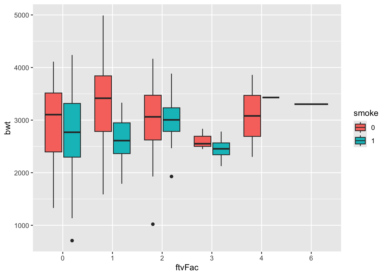 

5. Make a scatterplot with lwt on the \(x\)-axis and bwt on the \(y\)-axis. Modify the plot such that points are colored according to smoke and size shows ftv.

ggplot(birthData, aes(x=lwt, y=bwt, col=smoke, size = ftv)) +
  geom_point()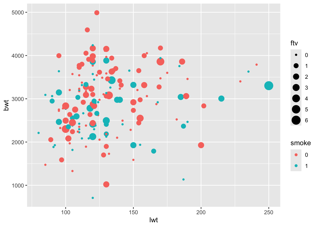 

6. The ftv is a numerical variable, but we would also like a categorical version of it called visits, with groups corresponding to zero visits, one visit, and two or more visits, respectively.

Hint

Use mutate and take a look at fct_collapse function.

    table(birthData$ftv)

  0   1   2   3   4   6 
100  47  30   7   4   1 

    birthData <- mutate(birthData, 
                        visits = fct_collapse(ftvFac, 
                                              Never="0", 
                                              Once="1", 
                                              other_level="MoreThanOnce"))
    table(birthData$visits)

       Never         Once MoreThanOnce 
         100           47           42 

7. Report how many women had more than one physician visit during the first trimester here.

   

Regression

The term regression is usually used for models where all explanatory variables are numerical.

If you are not too familiar with linear regression, you can have a look at what the summary() output means here and for understanding regression plot(), have a look here.

8. Fit a linear regression model with bwt as response and lwt as covariate, and identify the estimates for the intercept and for the slope. Find the 97.5% confidence interval for the slope parameter by using the confint() function.

library(ggplot2)
reg1 <- lm(bwt ~ lwt, data=birthData) 
summary(reg1)

Call:
lm(formula = bwt ~ lwt, data = birthData)

Residuals:
     Min       1Q   Median       3Q      Max 
-2192.12  -497.97    -3.84   508.32  2075.60 

Coefficients:
            Estimate Std. Error t value Pr(>|t|)    
(Intercept) 2369.624    228.493  10.371   <2e-16 ***
lwt            4.429      1.713   2.585   0.0105 *  
---
Signif. codes:  0 '***' 0.001 '**' 0.01 '*' 0.05 '.' 0.1 ' ' 1

Residual standard error: 718.4 on 187 degrees of freedom
Multiple R-squared:  0.0345,    Adjusted R-squared:  0.02933 
F-statistic: 6.681 on 1 and 187 DF,  p-value: 0.0105

confint(reg1)

                  2.5 %     97.5 %
(Intercept) 1918.867879 2820.37916
lwt            1.048845    7.80937

9. Perform model validation. Hint: use autoplot. Does the model seem appropriate for the data?

#par(mfrow=c(2,2))
#plot(reg1)
autoplot(reg1, which = 1:6, ncol = 2, label.size = 3)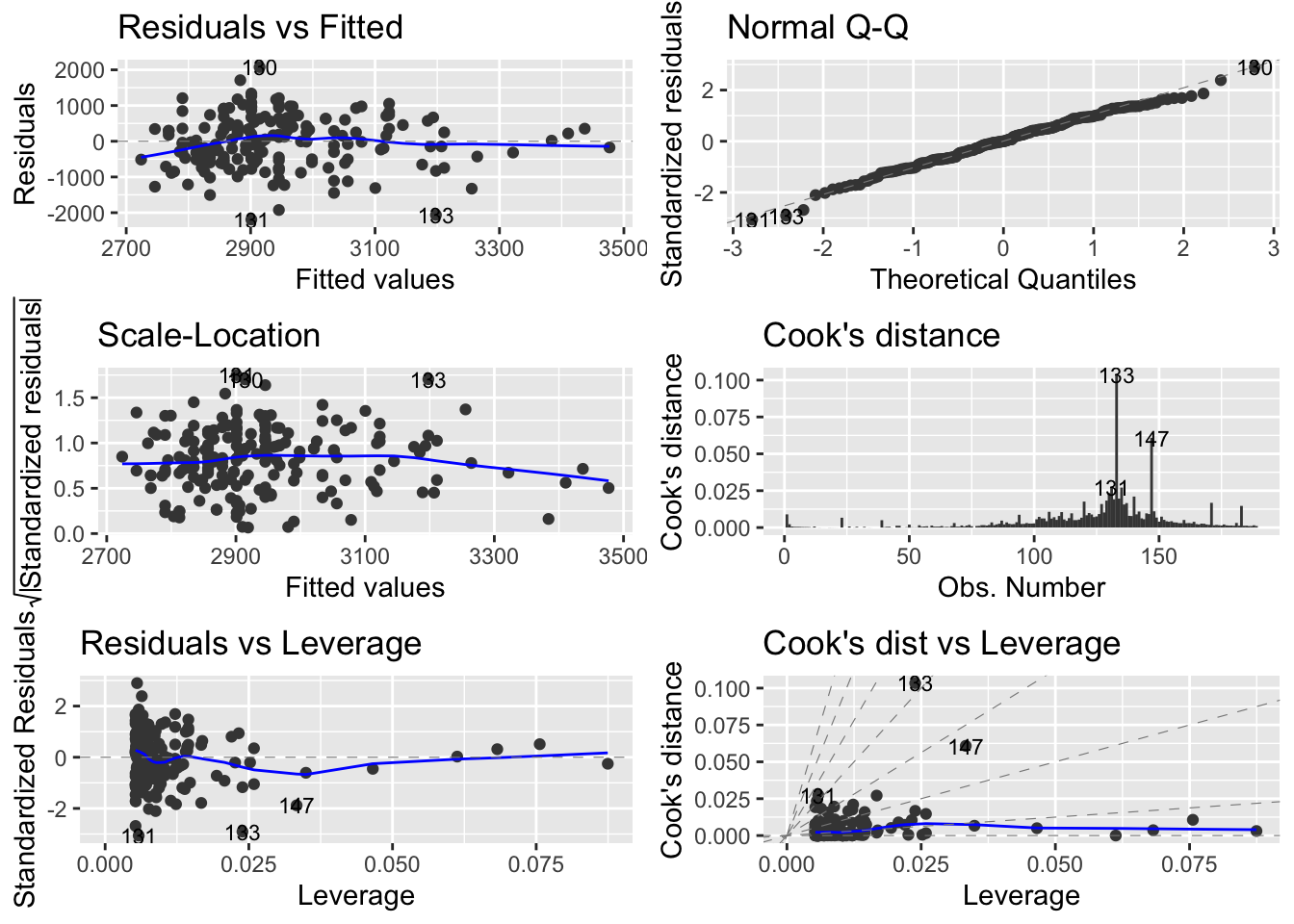

10. Fit the multiple linear regression model where you include lwt as well as age and ftv (numerical variables) as covariates. Identify the parameter estimates, and consider what their interpretation is.

reg2 <- lm(bwt ~ lwt + age + ftv, data=birthData)
summary(reg2)

Call:
lm(formula = bwt ~ lwt + age + ftv, data = birthData)

Residuals:
     Min       1Q   Median       3Q      Max 
-2218.60  -488.73    11.56   516.63  1907.42 

Coefficients:
            Estimate Std. Error t value Pr(>|t|)    
(Intercept) 2223.506    301.567   7.373  5.4e-12 ***
lwt            4.121      1.758   2.344   0.0201 *  
age            7.486     10.285   0.728   0.4676    
ftv           15.364     51.114   0.301   0.7641    
---
Signif. codes:  0 '***' 0.001 '**' 0.01 '*' 0.05 '.' 0.1 ' ' 1

Residual standard error: 720.9 on 185 degrees of freedom
Multiple R-squared:  0.03831,   Adjusted R-squared:  0.02271 
F-statistic: 2.457 on 3 and 185 DF,  p-value: 0.06446

# Just to view the coefficients
summary(reg2)$coefficients

               Estimate Std. Error   t value     Pr(>|t|)
(Intercept) 2223.505618 301.567140 7.3731694 5.402210e-12
lwt            4.120744   1.757787 2.3442798 2.012498e-02
age            7.485748  10.285178 0.7278189 4.676446e-01
ftv           15.363944  51.113921 0.3005824 7.640705e-01

11. Fit the multiple linear regression model again, but now only using data from mothers with a weight less than 160 pounds (lwt < 160). Hint: Use the filter function and change the data argument in the lm command.

    ### Use only data from mothers with weight below 160
    reg3 <- lm(bwt ~ lwt + age + ftv, data=filter(birthData, lwt<160))
    summary(reg3)

Call:
lm(formula = bwt ~ lwt + age + ftv, data = filter(birthData, 
    lwt < 160))

Residuals:
    Min      1Q  Median      3Q     Max 
-2233.9  -487.0    25.7   476.2  1852.5 

Coefficients:
            Estimate Std. Error t value Pr(>|t|)    
(Intercept) 1824.063    444.508   4.104 6.52e-05 ***
lwt            7.182      3.342   2.149   0.0332 *  
age            9.179     11.624   0.790   0.4310    
ftv           16.986     60.012   0.283   0.7775    
---
Signif. codes:  0 '***' 0.001 '**' 0.01 '*' 0.05 '.' 0.1 ' ' 1

Residual standard error: 716.3 on 157 degrees of freedom
Multiple R-squared:  0.03956,   Adjusted R-squared:  0.0212 
F-statistic: 2.155 on 3 and 157 DF,  p-value: 0.09549

    # Just to view the coefficients
    summary(reg3)$coefficients

               Estimate Std. Error   t value     Pr(>|t|)
(Intercept) 1824.063262 444.508301 4.1035528 0.0000651941
lwt            7.182184   3.341787 2.1492047 0.0331503757
age            9.178577  11.624301 0.7896024 0.4309508695
ftv           16.986307  60.011783 0.2830495 0.7775117320

ANOVA

The term analysis of variance (ANOVA) is used for models where all explanatory variables are categorical (factors). Before proceeding, make sure that smoke is coded as a factor.

12. Fit a one-way ANOVA (using lm()) where the mean birth weight is allowed to differ between smokers and non-smokers. Find the estimated birth weight for infants from smokers as well as non-smokers. Hint: use emmeans().

library(emmeans)    
oneway1 <- lm(bwt ~ smoke, data=birthData)
emmeans(oneway1,~smoke)

 smoke emmean   SE  df lower.CL upper.CL
 0       3056 66.9 187     2924     3188
 1       2772 83.4 187     2607     2937

Confidence level used: 0.95 

13. Check, is there a statistically significant difference in mean birth weight between infants of smokers and non-smokers?

pairs(emmeans(oneway1,~smoke))

 contrast        estimate  SE  df t.ratio p.value
 smoke0 - smoke1      284 107 187   2.653  0.0087

14. Fit the oneway ANOVA where you use visits as the explanatory variable. Perform an overall F-test for differences across all levels. Find the estimated birth weight for each group, and make the pairwise comparisons between the groups.
    Hint drop1(, test="F"). What do you conclude about the relationship between the number of visits and infant birth weight?

oneway2 <- lm(bwt ~ visits, data=birthData)
emmeans(oneway2,~visits)

 visits       emmean    SE  df lower.CL upper.CL
 Never          2865  72.6 186     2722     3008
 Once           3108 106.0 186     2899     3317
 MoreThanOnce   2951 112.0 186     2730     3172

Confidence level used: 0.95 

drop1(oneway2,test="F")

Single term deletions

Model:
bwt ~ visits
       Df Sum of Sq      RSS    AIC F value Pr(>F)
<none>              98081730 2493.2               
visits  2   1887925 99969656 2492.8  1.7901 0.1698

pairs(emmeans(oneway2,~visits))

 contrast             estimate  SE  df t.ratio p.value
 Never - Once           -242.9 128 186  -1.891  0.1441
 Never - MoreThanOnce    -85.7 134 186  -0.642  0.7970
 Once - MoreThanOnce     157.1 154 186   1.019  0.5658

P value adjustment: tukey method for comparing a family of 3 estimates 

15. Now, consider both visits and smoke as explanatory variables.
    Since both are categorical, the relevant model is a two-way ANOVA. Fit the model without interaction. Inspect the estimated means and group differences. How do you interpret the estimated means? What do they tell you about birth weight by smoking status and visit frequency?

twoway1 <- lm(bwt ~ visits + smoke, data=birthData)
emmeans(twoway1,~visits+smoke)

 visits       smoke emmean    SE  df lower.CL upper.CL
 Never        0       2981  86.7 185     2810     3152
 Once         0       3174 108.0 185     2960     3387
 MoreThanOnce 0       3055 119.0 185     2820     3290
 Never        1       2724  93.3 185     2540     2908
 Once         1       2916 132.0 185     2656     3177
 MoreThanOnce 1       2798 128.0 185     2545     3050

Confidence level used: 0.95 

pairs(emmeans(twoway1,~visits+smoke))

 contrast                                  estimate  SE  df t.ratio p.value
 Never smoke0 - Once smoke0                  -192.8 129 185  -1.499  0.6653
 Never smoke0 - MoreThanOnce smoke0           -74.1 132 185  -0.561  0.9933
 Never smoke0 - Never smoke1                  257.3 108 185   2.374  0.1709
 Never smoke0 - Once smoke1                    64.5 181 185   0.356  0.9992
 Never smoke0 - MoreThanOnce smoke1           183.2 174 185   1.054  0.8988
 Once smoke0 - MoreThanOnce smoke0            118.7 153 185   0.775  0.9715
 Once smoke0 - Never smoke1                   450.1 154 185   2.923  0.0444
 Once smoke0 - Once smoke1                    257.3 108 185   2.374  0.1709
 Once smoke0 - MoreThanOnce smoke1            376.0 178 185   2.112  0.2858
 MoreThanOnce smoke0 - Never smoke1           331.4 168 185   1.977  0.3596
 MoreThanOnce smoke0 - Once smoke1            138.6 197 185   0.704  0.9812
 MoreThanOnce smoke0 - MoreThanOnce smoke1    257.3 108 185   2.374  0.1709
 Never smoke1 - Once smoke1                  -192.8 129 185  -1.499  0.6653
 Never smoke1 - MoreThanOnce smoke1           -74.1 132 185  -0.561  0.9933
 Once smoke1 - MoreThanOnce smoke1            118.7 153 185   0.775  0.9715

P value adjustment: tukey method for comparing a family of 6 estimates 

16. Fit the twoway ANOVA model with interaction replacing + by a *. Use drop1() to test whether the interaction term is statistically significant. Compare it to model without interaction? What do the p-values suggest about whether the effect of smoking depends on the number of visits?

twoway2 <- lm(bwt ~ visits * smoke, data=birthData)
drop1(twoway2,test="F")

Single term deletions

Model:
bwt ~ visits * smoke
             Df Sum of Sq      RSS    AIC F value Pr(>F)
<none>                    93189162 2489.5               
visits:smoke  2   1992934 95182096 2489.5  1.9568 0.1443

drop1(twoway1,test="F")

Single term deletions

Model:
bwt ~ visits + smoke
       Df Sum of Sq      RSS    AIC F value  Pr(>F)  
<none>              95182096 2489.5                  
visits  2   1161614 96343710 2487.8  1.1289 0.32561  
smoke   1   2899635 98081730 2493.2  5.6359 0.01862 *
---
Signif. codes:  0 '***' 0.001 '**' 0.01 '*' 0.05 '.' 0.1 ' ' 1

17. Use anova() to formally compare the two models. Are the two models statistically different?
    What does this imply about including the interaction term?

anova(twoway1, twoway2)

Analysis of Variance Table

Model 1: bwt ~ visits + smoke
Model 2: bwt ~ visits * smoke
  Res.Df      RSS Df Sum of Sq      F Pr(>F)
1    185 95182096                           
2    183 93189162  2   1992934 1.9568 0.1443

18. Report are the 2 models statistically different here.

Optional section

Logistic regression

19. The variable low is 1 if birth weight is less than 2500 g, and 0 otherwise.
    Visualize the data:

ggplot(birthData, aes(x=bwt, y=low)) + 
  geom_point() +
  labs(y = "Low birthweight (1 = yes, 0 = no)")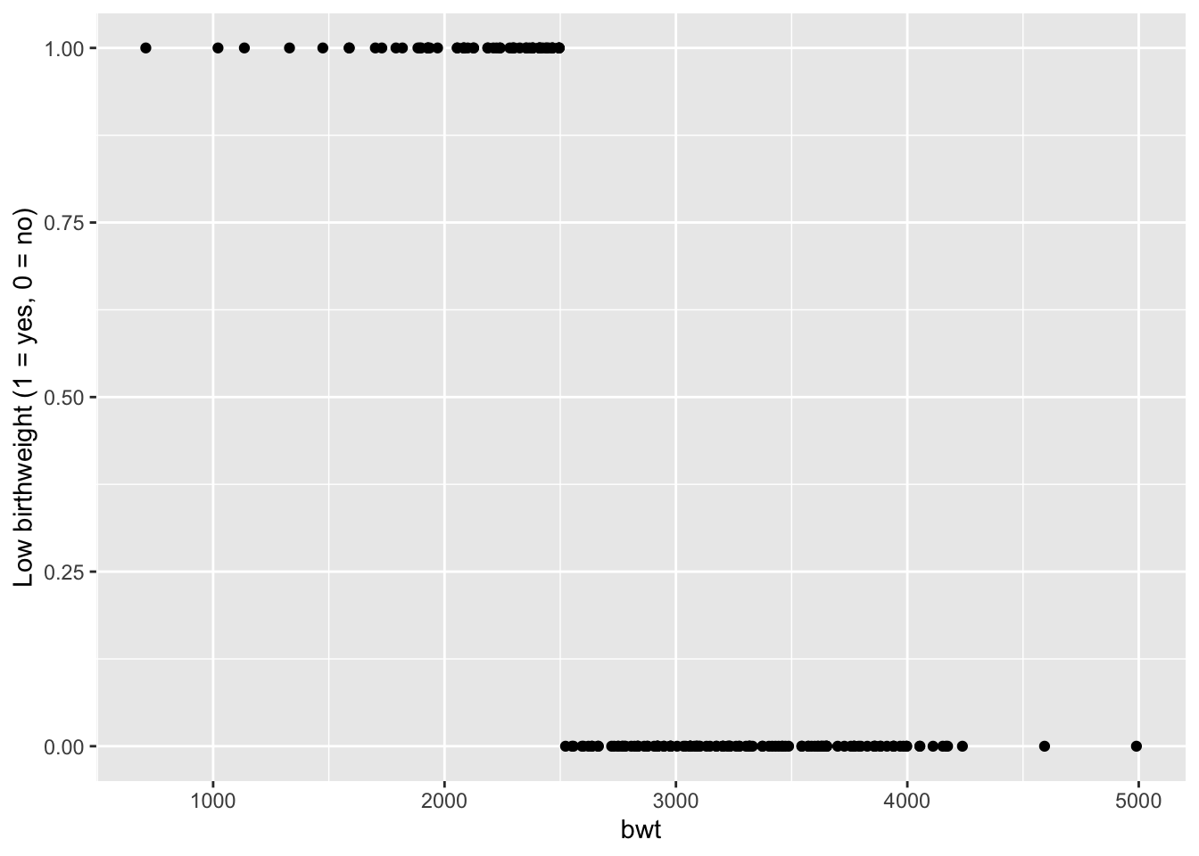

Imagine the actual birth weight bwt was not recorded, but we still want to know whether the birth weight was low.
Because the outcome is binary (low has two values), we use logistic regression to model the probability.

For example, we may consider a model with mothers’s weight, smoking status, and age as predictors, just like in the previous question.

20. Fit the model, take a look at glm function:

logreg1 <- glm(low ~ lwt + smoke + age, 
               data=birthData, family="binomial")
logreg1

Call:  glm(formula = low ~ lwt + smoke + age, family = "binomial", data = birthData)

Coefficients:
(Intercept)          lwt       smoke1          age  
    1.36823     -0.01214      0.67076     -0.03899  

Degrees of Freedom: 188 Total (i.e. Null);  185 Residual
Null Deviance:      234.7 
Residual Deviance: 222.9    AIC: 230.9

21. Use drop1() to check if each predictor contributes significantly:

    A Note: test = "F" is for Gaussian linear models (lm()), where F-tests are appropriate.
    For logistic regression and other GLMs, test = "Chisq" is the correct choice.

drop1(logreg1, test="Chisq")

Single term deletions

Model:
low ~ lwt + smoke + age
       Df Deviance    AIC    LRT Pr(>Chi)  
<none>      222.88 230.88                  
lwt     1   227.28 233.28 4.3969  0.03600 *
smoke   1   227.12 233.12 4.2440  0.03939 *
age     1   224.34 230.34 1.4613  0.22672  
---
Signif. codes:  0 '***' 0.001 '**' 0.01 '*' 0.05 '.' 0.1 ' ' 1

**Question:** Based on the p-values, is there evidence that **smoking** affects the probability of low birth weight?

22. The fitted model may be used to predict the outcome for new values. The new values are provided in a newData data frame with the same names as the covariate in the model. 

# new data
newData <- tibble(
    low = rep(NA, 5),
    age = c(22, 30, 18, 17, 28),
    lwt = c(140, 155, 130, 97, 165),
    race = c("Black", "Other", "Black", "Other", "White"),
    smoke = as.factor(c(1, 0, 1, 1, 0)),
    ptl = c(1, 0, 0, 0, 0),
    ftv = c(1, 3, 0, 0, 2),
    bwt = c(2800, 4500, 1700, 1500, 3400)
    )

23. We have data for 5 new mothers. Use your fitted logistic model logreg1 to predict the probability of low birthweight and fill the low column. Use the predict() function to compute the predicted probabilities for the new cases. Make sure to set type="response" to get probabilities rather than log-odds.

newData$low <- predict(logreg1, 
                       newdata = newData, 
                       type = "response")

24. Add the predicted probabilities (red points) and a connecting line to your ggplot. Hint: add geom_point and geom_line with the newData.

ggplot(birthData, aes(x=bwt, y=low)) + 
  geom_point() +
  geom_point(data = newData, aes(x = bwt, y = low), color = "red", size = 2) +
  geom_line(data = newData, aes(x = bwt, y = low), color = "red", size = 0.5) +
      labs(y = "Predicted probability of low birthweight")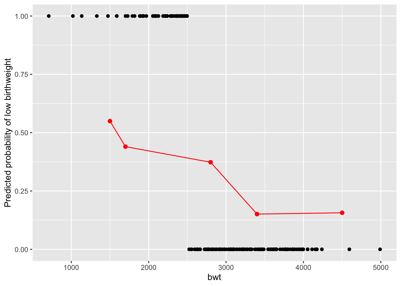

25. Report here - In how many of the new cases is birthweight predicted to be low??